Cluster analysis

Part of a series on
Machine learning and data mining
Paradigms Supervised learning Unsupervised learning Online learning Batch learning Meta-learning Semi-supervised learning Self-supervised learning Reinforcement learning Curriculum learning Rule-based learning Quantum machine learning
Problems Classification Generative modeling Regression Clustering Dimensionality reduction Density estimation Anomaly detection Data cleaning AutoML Association rules Semantic analysis Structured prediction Feature engineering Feature learning Learning to rank Grammar induction Ontology learning Multimodal learning
Supervised learning (classification • regression) Apprenticeship learning Decision trees Ensembles Bagging Boosting Random forest k-NN Linear regression Naive Bayes Artificial neural networks Logistic regression Perceptron Relevance vector machine (RVM) Support vector machine (SVM)
Clustering BIRCH CURE Hierarchical k-means Fuzzy Expectation–maximization (EM) DBSCAN OPTICS Mean shift
Dimensionality reduction Factor analysis CCA ICA LDA NMF PCA PGD t-SNE SDL
Structured prediction Graphical models Bayes net Conditional random field Hidden Markov
Anomaly detection RANSAC k-NN Local outlier factor Isolation forest
Artificial neural network Autoencoder Cognitive computing Deep learning DeepDream Feedforward neural network Recurrent neural network LSTM GRU ESN reservoir computing Restricted Boltzmann machine GAN Diffusion model SOM Convolutional neural network U-Net Transformer Vision Mamba Spiking neural network Memtransistor Electrochemical RAM (ECRAM)
Reinforcement learning Q-learning SARSA Temporal difference (TD) Multi-agent Self-play
Learning with humans Active learning Crowdsourcing Human-in-the-loop RLHF
Model diagnostics Coefficient of determination Confusion matrix Learning curve ROC curve
Mathematical foundations Kernel machines Bias–variance tradeoff Computational learning theory Empirical risk minimization Occam learning PAC learning Statistical learning VC theory
Machine-learning venues ECML PKDD NeurIPS ICML ICLR IJCAI ML JMLR
Related articles Glossary of artificial intelligence List of datasets for machine-learning research List of datasets in computer vision and image processing Outline of machine learning
v t e

Cluster analysis or clustering is the task of grouping a set of objects in such a way that objects in the same group (called a cluster) are more similar (in some specific sense defined by the analyst) to each other than to those in other groups (clusters). It is a main task of exploratory data analysis, and a common technique for statistical data analysis, used in many fields, including pattern recognition, image analysis, information retrieval, bioinformatics, data compression, computer graphics and machine learning.

Cluster analysis refers to a family of algorithms and tasks rather than one specific

and model parameters until the result achieves the desired properties.

Besides the term clustering, there is a number of terms with similar meanings, including automatic classification, numerical taxonomy, botryology (from Greek: βότρυς 'grape'), typological analysis, and community detection. The subtle differences are often in the use of the results: while in data mining, the resulting groups are the matter of interest, in automatic classification the resulting discriminative power is of interest.

Cluster analysis was originated in anthropology by Driver and Kroeber in 1932^[1] and introduced to psychology by Joseph Zubin in 1938^[2] and Robert Tryon in 1939^[3] and famously used by Cattell beginning in 1943^[4] for trait theory classification in personality psychology.

Definition

The notion of a "cluster" cannot be precisely defined, which is one of the reasons why there are so many clustering algorithms.^[5] There is a common denominator: a group of data objects. However, different researchers employ different cluster models, and for each of these cluster models again different algorithms can be given. The notion of a cluster, as found by different algorithms, varies significantly in its properties. Understanding these "cluster models" is key to understanding the differences between the various algorithms. Typical cluster models include:

• Connectivity models: for example, hierarchical clustering builds models based on distance connectivity.
• Centroid models: for example, the
  k-means algorithm
  represents each cluster by a single mean vector.
• Distribution models: clusters are modeled using statistical distributions, such as
  expectation-maximization algorithm
  .
• Density models: for example,
  OPTICS
  defines clusters as connected dense regions in the data space.
• Subspace models: in biclustering (also known as co-clustering or two-mode-clustering), clusters are modeled with both cluster members and relevant attributes.
• Group models: some algorithms do not provide a refined model for their results and just provide the grouping information.
• Graph-based models: a clique, that is, a subset of nodes in a graph such that every two nodes in the subset are connected by an edge can be considered as a prototypical form of cluster. Relaxations of the complete connectivity requirement (a fraction of the edges can be missing) are known as quasi-cliques, as in the HCS clustering algorithm.
• Signed graph models: Every path in a signed graph has a sign from the product of the signs on the edges. Under the assumptions of balance theory, edges may change sign and result in a bifurcated graph. The weaker "clusterability axiom" (no cycle has exactly one negative edge) yields results with more than two clusters, or subgraphs with only positive edges.^[6]
• Neural models: the most well-known
  Independent Component Analysis
  .

A "clustering" is essentially a set of such clusters, usually containing all objects in the data set. Additionally, it may specify the relationship of the clusters to each other, for example, a hierarchy of clusters embedded in each other. Clusterings can be roughly distinguished as:

• Hard clustering: each object belongs to a cluster or not
• Soft clustering (also: fuzzy clustering): each object belongs to each cluster to a certain degree (for example, a likelihood of belonging to the cluster)

There are also finer distinctions possible, for example:

• Strict partitioning clustering: each object belongs to exactly one cluster
• Strict partitioning clustering with outliers: objects can also belong to no cluster; in which case they are considered outliers
• Overlapping clustering (also: alternative clustering, multi-view clustering): objects may belong to more than one cluster; usually involving hard clusters
• Hierarchical clustering: objects that belong to a child cluster also belong to the parent cluster
• Subspace clustering
  : while an overlapping clustering, within a uniquely defined subspace, clusters are not expected to overlap

Algorithms

As listed above, clustering algorithms can be categorized based on their cluster model. The following overview will only list the most prominent examples of clustering algorithms, as there are possibly over 100 published clustering algorithms. Not all provide models for their clusters and can thus not easily be categorized. An overview of algorithms explained in Wikipedia can be found in the list of statistics algorithms.

There is no objectively "correct" clustering algorithm, but as it was noted, "clustering is in the eye of the beholder."^[5] The most appropriate clustering algorithm for a particular problem often needs to be chosen experimentally, unless there is a mathematical reason to prefer one cluster model over another. An algorithm that is designed for one kind of model will generally fail on a data set that contains a radically different kind of model.^[5] For example, k-means cannot find non-convex clusters.^[5] Most traditional clustering methods assume the clusters exhibit a spherical, elliptical or convex shape.^[7]

Connectivity-based clustering (hierarchical clustering)

Connectivity-based clustering, also known as hierarchical clustering, is based on the core idea of objects being more related to nearby objects than to objects farther away. These algorithms connect "objects" to form "clusters" based on their distance. A cluster can be described largely by the maximum distance needed to connect parts of the cluster. At different distances, different clusters will form, which can be represented using a dendrogram, which explains where the common name "hierarchical clustering" comes from: these algorithms do not provide a single partitioning of the data set, but instead provide an extensive hierarchy of clusters that merge with each other at certain distances. In a dendrogram, the y-axis marks the distance at which the clusters merge, while the objects are placed along the x-axis such that the clusters don't mix.

Connectivity-based clustering is a whole family of methods that differ by the way distances are computed. Apart from the usual choice of

("Unweighted or Weighted Pair Group Method with Arithmetic Mean", also known as average linkage clustering). Furthermore, hierarchical clustering can be agglomerative (starting with single elements and aggregating them into clusters) or divisive (starting with the complete data set and dividing it into partitions).

These methods will not produce a unique partitioning of the data set, but a hierarchy from which the user still needs to choose appropriate clusters. They are not very robust towards outliers, which will either show up as additional clusters or even cause other clusters to merge (known as "chaining phenomenon", in particular with single-linkage clustering). In the general case, the complexity is ${\displaystyle {\mathcal {O}}(n^{3})}$ for agglomerative clustering and ${\displaystyle {\mathcal {O}}(2^{n-1})}$ for

which makes them too slow for large data sets. For some special cases, optimal efficient methods (of complexity ${\displaystyle {\mathcal {O}}(n^{2})}$) are known: SLINK[9] for single-linkage and CLINK^[10] for complete-linkage clustering.

• Linkage clustering examples
• 
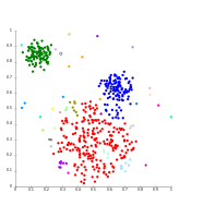  Single-linkage on Gaussian data. At 35 clusters, the biggest cluster starts fragmenting into smaller parts, while before it was still connected to the second largest due to the single-link effect.
• 
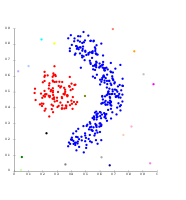  Single-linkage on density-based clusters. 20 clusters extracted, most of which contain single elements, since linkage clustering does not have a notion of "noise".

Centroid-based clustering

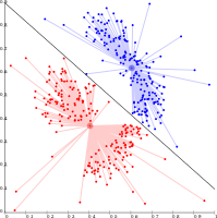
In centroid-based clustering, each cluster is represented by a central vector, which is not necessarily a member of the data set. When the number of clusters is fixed to k, k-means clustering gives a formal definition as an optimization problem: find the k cluster centers and assign the objects to the nearest cluster center, such that the squared distances from the cluster are minimized.

The optimization problem itself is known to be

).

Most k-means-type algorithms require the number of clusters – k – to be specified in advance, which is considered to be one of the biggest drawbacks of these algorithms. Furthermore, the algorithms prefer clusters of approximately similar size, as they will always assign an object to the nearest centroid. This often leads to incorrectly cut borders of clusters (which is not surprising since the algorithm optimizes cluster centers, not cluster borders).

K-means has a number of interesting theoretical properties. First, it partitions the data space into a structure known as a

for this model discussed below.

• k-means clustering examples
• 
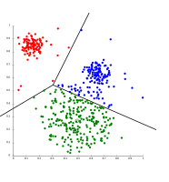  k-means separates data into Voronoi cells, which assumes equal-sized clusters (not adequate here).
• 
  k-means cannot represent density-based clusters.

Centroid-based clustering problems such as k-means and k-medoids are special cases of the uncapacitated, metric facility location problem, a canonical problem in the operations research and computational geometry communities. In a basic facility location problem (of which there are numerous variants that model more elaborate settings), the task is to find the best warehouse locations to optimally service a given set of consumers. One may view "warehouses" as cluster centroids and "consumer locations" as the data to be clustered. This makes it possible to apply the well-developed algorithmic solutions from the facility location literature to the presently considered centroid-based clustering problem.

Model-based clustering

The clustering framework most closely related to statistics is model-based clustering, which is based on distribution models. This approach models the data as arising from a mixture of probability distributions. It has the advantages of providing principled statistical answers to questions such as how many clusters there are, what clustering method or model to use, and how to detect and deal with outliers.

While the theoretical foundation of these methods is excellent, they suffer from

of the covariance matrices, that provide a balance between overfitting and fidelity to the data.

One prominent method is known as Gaussian mixture models (using the

, so multiple runs may produce different results. In order to obtain a hard clustering, objects are often then assigned to the Gaussian distribution they most likely belong to; for soft clusterings, this is not necessary.

Distribution-based clustering produces complex models for clusters that can capture

between attributes. However, these algorithms put an extra burden on the user: for many real data sets, there may be no concisely defined mathematical model (e.g. assuming Gaussian distributions is a rather strong assumption on the data).

• Gaussian mixture model clustering examples
• 
  On Gaussian-distributed data, EM works well, since it uses Gaussians for modelling clusters.
• 
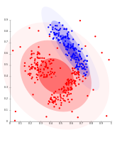  Density-based clusters cannot be modeled using Gaussian distributions.

Density-based clustering

In density-based clustering,^[12] clusters are defined as areas of higher density than the remainder of the data set. Objects in sparse areas – that are required to separate clusters – are usually considered to be noise and border points.

The most popular^[13] density-based clustering method is DBSCAN.^[14] In contrast to many newer methods, it features a well-defined cluster model called "density-reachability". Similar to linkage-based clustering, it is based on connecting points within certain distance thresholds. However, it only connects points that satisfy a density criterion, in the original variant defined as a minimum number of other objects within this radius. A cluster consists of all density-connected objects (which can form a cluster of an arbitrary shape, in contrast to many other methods) plus all objects that are within these objects' range. Another interesting property of DBSCAN is that its complexity is fairly low – it requires a linear number of range queries on the database – and that it will discover essentially the same results (it is deterministic for core and noise points, but not for border points) in each run, therefore there is no need to run it multiple times. OPTICS^[15] is a generalization of DBSCAN that removes the need to choose an appropriate value for the range parameter ${\displaystyle \varepsilon }$, and produces a hierarchical result related to that of linkage clustering. DeLi-Clu,^[16] Density-Link-Clustering combines ideas from single-linkage clustering and OPTICS, eliminating the ${\displaystyle \varepsilon }$ parameter entirely and offering performance improvements over OPTICS by using an R-tree index.

The key drawback of

that are able to precisely model this kind of data.

• Density-based clustering examples
• 
  Density-based clustering with DBSCAN
• 
  DBSCAN assumes clusters of similar density, and may have problems separating nearby clusters.
• 
  OPTICS is a DBSCAN variant, improving handling of different densities clusters.

Grid-based clustering

The grid-based technique is used for a multi-dimensional data set.^[17] In this technique, we create a grid structure, and the comparison is performed on grids (also known as cells). The grid-based technique is fast and has low computational complexity. There are two types of grid-based clustering methods: STING and CLIQUE. Steps involved in grid-based clustering algorithm are:

1. Divide data space into a finite number of cells.
2. Randomly select a cell ‘c’, where c should not be traversed beforehand.
3. Calculate the density of ‘c’
4. If the density of ‘c’ greater than threshold density
   1. Mark cell ‘c’ as a new cluster
   2. Calculate the density of all the neighbors of ‘c’
   3. If the density of a neighboring cell is greater than threshold density then, add the cell in the cluster and repeat steps 4.2 and 4.3 till there is no neighbor with a density greater than threshold density.
5. Repeat steps 2,3 and 4 till all the cells are traversed.
6. Stop.

Recent developments

In recent years, considerable effort has been put into improving the performance of existing algorithms.

.

For

Ideas from density-based clustering methods (in particular the

exploring hierarchical density-based correlation clusters).

Several different clustering systems based on

Evaluation and assessment

Evaluation (or "validation") of clustering results is as difficult as the clustering itself.[34] Popular approaches involve "internal" evaluation, where the clustering is summarized to a single quality score, "external" evaluation, where the clustering is compared to an existing "ground truth" classification, "manual" evaluation by a human expert, and "indirect" evaluation by evaluating the utility of the clustering in its intended application.^[35]

Internal evaluation measures suffer from the problem that they represent functions that themselves can be seen as a clustering objective. For example, one could cluster the data set by the Silhouette coefficient; except that there is no known efficient algorithm for this. By using such an internal measure for evaluation, one rather compares the similarity of the optimization problems,^[35] and not necessarily how useful the clustering is.

External evaluation has similar problems: if we have such "ground truth" labels, then we would not need to cluster; and in practical applications we usually do not have such labels. On the other hand, the labels only reflect one possible partitioning of the data set, which does not imply that there does not exist a different, and maybe even better, clustering.

Neither of these approaches can therefore ultimately judge the actual quality of a clustering, but this needs human evaluation,^[35] which is highly subjective. Nevertheless, such statistics can be quite informative in identifying bad clusterings,^[36] but one should not dismiss subjective human evaluation.^[36]

Internal evaluation

When a clustering result is evaluated based on the data that was clustered itself, this is called internal evaluation. These methods usually assign the best score to the algorithm that produces clusters with high similarity within a cluster and low similarity between clusters. One drawback of using internal criteria in cluster evaluation is that high scores on an internal measure do not necessarily result in effective information retrieval applications.^[37] Additionally, this evaluation is biased towards algorithms that use the same cluster model. For example, k-means clustering naturally optimizes object distances, and a distance-based internal criterion will likely overrate the resulting clustering.

Therefore, the internal evaluation measures are best suited to get some insight into situations where one algorithm performs better than another, but this shall not imply that one algorithm produces more valid results than another.^[5] Validity as measured by such an index depends on the claim that this kind of structure exists in the data set. An algorithm designed for some kind of models has no chance if the data set contains a radically different set of models, or if the evaluation measures a radically different criterion.^[5] For example, k-means clustering can only find convex clusters, and many evaluation indexes assume convex clusters. On a data set with non-convex clusters neither the use of k-means, nor of an evaluation criterion that assumes convexity, is sound.

More than a dozen of internal evaluation measures exist, usually based on the intuition that items in the same cluster should be more similar than items in different clusters.^{[38]: 115–121} For example, the following methods can be used to assess the quality of clustering algorithms based on internal criterion:

• Davies–Bouldin index

The Davies–Bouldin index can be calculated by the following formula:

${\displaystyle DB={\frac {1}{n}}\sum _{i=1}^{n}\max _{j\neq i}\left({\frac {\sigma _{i}+\sigma _{j}}{d(c_{i},c_{j})}}\right)}$

where n is the number of clusters, ${\displaystyle c_{i}}$ is the centroid of cluster ${\displaystyle i}$, ${\displaystyle \sigma _{i}}$ is the average distance of all elements in cluster ${\displaystyle i}$ to centroid ${\displaystyle c_{i}}$, and ${\displaystyle d(c_{i},c_{j})}$ is the distance between centroids ${\displaystyle c_{i}}$ and ${\displaystyle c_{j}}$. Since algorithms that produce clusters with low intra-cluster distances (high intra-cluster similarity) and high inter-cluster distances (low inter-cluster similarity) will have a low Davies–Bouldin index, the clustering algorithm that produces a collection of clusters with the smallest Davies–Bouldin index is considered the best algorithm based on this criterion.

• Dunn index

The Dunn index aims to identify dense and well-separated clusters. It is defined as the ratio between the minimal inter-cluster distance to maximal intra-cluster distance. For each cluster partition, the Dunn index can be calculated by the following formula:^[39]

${\displaystyle D={\frac {\min _{1\leq i<j\leq n}d(i,j)}{\max _{1\leq k\leq n}d^{\prime }(k)}}\,,}$

where d(i,j) represents the distance between clusters i and j, and d '(k) measures the intra-cluster distance of cluster k. The inter-cluster distance d(i,j) between two clusters may be any number of distance measures, such as the distance between the

centroids

of the clusters. Similarly, the intra-cluster distance d '(k) may be measured in a variety of ways, such as the maximal distance between any pair of elements in cluster k. Since internal criterion seek clusters with high intra-cluster similarity and low inter-cluster similarity, algorithms that produce clusters with high Dunn index are more desirable.

• Silhouette coefficient

The silhouette coefficient contrasts the average distance to elements in the same cluster with the average distance to elements in other clusters. Objects with a high silhouette value are considered well clustered, objects with a low value may be outliers. This index works well with k-means clustering,^{[citation needed]} and is also used to determine the optimal number of clusters.

External evaluation

In external evaluation, clustering results are evaluated based on data that was not used for clustering, such as known class labels and external benchmarks. Such benchmarks consist of a set of pre-classified items, and these sets are often created by (expert) humans. Thus, the benchmark sets can be thought of as a

A number of measures are adapted from variants used to evaluate classification tasks. In place of counting the number of times a class was correctly assigned to a single data point (known as

As with internal evaluation, several external evaluation measures exist,[38]^{: 125–129} for example:

• Purity: Purity is a measure of the extent to which clusters contain a single class.^[37] Its calculation can be thought of as follows: For each cluster, count the number of data points from the most common class in said cluster. Now take the sum over all clusters and divide by the total number of data points. Formally, given some set of clusters ${\displaystyle M}$ and some set of classes ${\displaystyle D}$, both partitioning ${\displaystyle N}$ data points, purity can be defined as:

${\displaystyle {\frac {1}{N}}\sum _{m\in M}\max _{d\in D}{|m\cap d|}}$

This measure doesn't penalize having many clusters, and more clusters will make it easier to produce a high purity. A purity score of 1 is always possible by putting each data point in its own cluster. Also, purity doesn't work well for imbalanced data, where even poorly performing clustering algorithms will give a high purity value. For example, if a size 1000 dataset consists of two classes, one containing 999 points and the other containing 1 point, then every possible partition will have a purity of at least 99.9%.

• Rand index^[42]

The Rand index computes how similar the clusters (returned by the clustering algorithm) are to the benchmark classifications. It can be computed using the following formula:

${\displaystyle RI={\frac {TP+TN}{TP+FP+FN+TN}}}$

where ${\displaystyle TP}$ is the number of true positives, ${\displaystyle TN}$ is the number of

true negatives

, ${\displaystyle FP}$ is the number of

false positives

, and ${\displaystyle FN}$ is the number of

false negatives

. The instances being counted here are the number of correct pairwise assignments. That is, ${\displaystyle TP}$ is the number of pairs of points that are clustered together in the predicted partition and in the ground truth partition, ${\displaystyle FP}$ is the number of pairs of points that are clustered together in the predicted partition but not in the ground truth partition etc. If the dataset is of size N, then ${\displaystyle TP+TN+FP+FN={\binom {N}{2}}}$.

One issue with the

.

• F-measure

The F-measure can be used to balance the contribution of

recall

through a parameter ${\displaystyle \beta \geq 0}$. Let

recall

(both external evaluation measures in themselves) be defined as follows:

${\displaystyle P={\frac {TP}{TP+FP}}}$

${\displaystyle R={\frac {TP}{TP+FN}}}$

where ${\displaystyle P}$ is the

precision

rate and ${\displaystyle R}$ is the

recall rate. We can calculate the F-measure by using the following formula:^[37]

${\displaystyle F_{\beta }={\frac {(\beta ^{2}+1)\cdot P\cdot R}{\beta ^{2}\cdot P+R}}}$

When ${\displaystyle \beta =0}$, ${\displaystyle F_{0}=P}$. In other words,

recall

has no impact on the F-measure when ${\displaystyle \beta =0}$, and increasing ${\displaystyle \beta }$ allocates an increasing amount of weight to recall in the final F-measure.

Also ${\displaystyle TN}$ is not taken into account and can vary from 0 upward without bound.

• Jaccard index

The Jaccard index is used to quantify the similarity between two datasets. The

Jaccard index

takes on a value between 0 and 1. An index of 1 means that the two dataset are identical, and an index of 0 indicates that the datasets have no common elements. The Jaccard index is defined by the following formula:

${\displaystyle J(A,B)={\frac {|A\cap B|}{|A\cup B|}}={\frac {TP}{TP+FP+FN}}}$

This is simply the number of unique elements common to both sets divided by the total number of unique elements in both sets.

Note that ${\displaystyle TN}$ is not taken into account.

• Dice index

The Dice symmetric measure doubles the weight on ${\displaystyle TP}$ while still ignoring ${\displaystyle TN}$:

${\displaystyle DSC={\frac {2TP}{2TP+FP+FN}}}$

• Fowlkes–Mallows index^[43]

The Fowlkes–Mallows index computes the similarity between the clusters returned by the clustering algorithm and the benchmark classifications. The higher the value of the Fowlkes–Mallows index the more similar the clusters and the benchmark classifications are. It can be computed using the following formula:

${\displaystyle FM={\sqrt {{\frac {TP}{TP+FP}}\cdot {\frac {TP}{TP+FN}}}}}$

where ${\displaystyle TP}$ is the number of

true positives

, ${\displaystyle FP}$ is the number of

false positives

, and ${\displaystyle FN}$ is the number of

false negatives

. The ${\displaystyle FM}$ index is the geometric mean of the

recall

${\displaystyle P}$ and ${\displaystyle R}$, and is thus also known as the G-measure, while the F-measure is their harmonic mean.

recall

are also known as Wallace's indices ${\displaystyle B^{I}}$ and ${\displaystyle B^{II}}$.

Matthews Correlation and relate strongly to Kappa.^[47]

• Chi Index[48] is an external validation index that measure the clustering results by applying the chi-squared statistic. This index scores positively the fact that the labels are as sparse as possible across the clusters, i.e., that each cluster has as few different labels as possible. The higher the value of the Chi Index the greater the relationship between the resulting clusters and the label used.
• The mutual information is an information theoretic measure of how much information is shared between a clustering and a ground-truth classification that can detect a non-linear similarity between two clusterings. Normalized mutual information is a family of corrected-for-chance variants of this that has a reduced bias for varying cluster numbers.^[34]
• Confusion matrix

A confusion matrix can be used to quickly visualize the results of a classification (or clustering) algorithm. It shows how different a cluster is from the gold standard cluster.

Cluster tendency

To measure cluster tendency is to measure to what degree clusters exist in the data to be clustered, and may be performed as an initial test, before attempting clustering. One way to do this is to compare the data against random data. On average, random data should not have clusters.

• Hopkins statistic

There are multiple formulations of the Hopkins statistic.^[49] A typical one is as follows.^[50] Let ${\displaystyle X}$ be the set of ${\displaystyle n}$ data points in ${\displaystyle d}$ dimensional space. Consider a random sample (without replacement) of ${\displaystyle m\ll n}$ data points with members ${\displaystyle x_{i}}$. Also generate a set ${\displaystyle Y}$ of ${\displaystyle m}$ uniformly randomly distributed data points. Now define two distance measures, ${\displaystyle u_{i}}$ to be the distance of ${\displaystyle y_{i}\in Y}$ from its nearest neighbor in X and ${\displaystyle w_{i}}$ to be the distance of ${\displaystyle x_{i}\in X}$ from its nearest neighbor in X. We then define the Hopkins statistic as:

${\displaystyle H={\frac {\sum _{i=1}^{m}{u_{i}^{d}}}{\sum _{i=1}^{m}{u_{i}^{d}}+\sum _{i=1}^{m}{w_{i}^{d}}}}\,,}$

With this definition, uniform random data should tend to have values near to 0.5, and clustered data should tend to have values nearer to 1.

However, data containing just a single Gaussian will also score close to 1, as this statistic measures deviation from a uniform distribution, not multimodality, making this statistic largely useless in application (as real data never is remotely uniform).

Applications

This section needs additional citations for verification. Please help improve this article by adding citations to reliable sources in this section. Unsourced material may be challenged and removed. (November 2016) (Learn how and when to remove this template message)

Biology, computational biology and bioinformatics

Plant and animal ecology

Cluster analysis is used to describe and to make spatial and temporal comparisons of communities (assemblages) of organisms in heterogeneous environments. It is also used in

phylogenies

or clusters of organisms (individuals) at the species, genus or higher level that share a number of attributes.

Transcriptomics

Clustering is used to build groups of

genome annotation – a general aspect of genomics

.

Sequence analysis

Sequence clustering is used to group homologous sequences into gene families.^[53] This is a very important concept in bioinformatics, and evolutionary biology in general. See evolution by gene duplication.

High-throughput genotyping platforms

Clustering algorithms are used to automatically assign genotypes.^[54]

Human genetic clustering

The similarity of genetic data is used in clustering to infer population structures.

Medicine

Medical imaging

On

PET scans, cluster analysis can be used to differentiate between different types of tissue in a three-dimensional image for many different purposes.^[55]

Analysis of antimicrobial activity

Cluster analysis can be used to analyse patterns of antibiotic resistance, to classify antimicrobial compounds according to their mechanism of action, to classify antibiotics according to their antibacterial activity.

IMRT segmentation

Clustering can be used to divide a fluence map into distinct regions for conversion into deliverable fields in MLC-based Radiation Therapy.

Business and marketing

Market research

Cluster analysis is widely used in market research when working with multivariate data from

customers, and for use in market segmentation, product positioning, new product development

and selecting test markets.

Grouping of shopping items

Clustering can be used to group all the shopping items available on the web into a set of unique products. For example, all the items on eBay can be grouped into unique products (eBay does not have the concept of a

SKU

).

World Wide Web

Social network analysis

In the study of

communities

within large groups of people.

Search result grouping

In the process of intelligent grouping of the files and websites, clustering may be used to create a more relevant set of search results compared to normal search engines like

Clusty. It also may be used to return a more comprehensive set of results in cases where a search term could refer to vastly different things. Each distinct use of the term corresponds to a unique cluster of results, allowing a ranking algorithm to return comprehensive results by picking the top result from each cluster.^[56]

Slippy map optimization

Flickr's map of photos and other map sites use clustering to reduce the number of markers on a map.^{[citation needed]} This makes it both faster and reduces the amount of visual clutter.

Computer science

Software evolution

Clustering is useful in software evolution as it helps to reduce legacy properties in code by reforming functionality that has become dispersed. It is a form of restructuring and hence is a way of direct preventative maintenance.

Image segmentation

Clustering can be used to divide a

object recognition.^[57]

Evolutionary algorithms

Clustering may be used to identify different niches within the population of an evolutionary algorithm so that reproductive opportunity can be distributed more evenly amongst the evolving species or subspecies.

Recommender systems

Recommender systems are designed to recommend new items based on a user's tastes. They sometimes use clustering algorithms to predict a user's preferences based on the preferences of other users in the user's cluster.

Markov chain Monte Carlo methods

Clustering is often utilized to locate and characterize extrema in the target distribution.

Anomaly detection

Anomalies/outliers are typically – be it explicitly or implicitly – defined with respect to clustering structure in data.

Natural language processing

Clustering can be used to resolve

lexical ambiguity.^[56]

DevOps

Clustering has been used to analyse the effectiveness of DevOps teams.^[58]

Social science

Sequence analysis in social sciences

Cluster analysis is used to identify patterns of family life trajectories, professional careers, and daily or weekly time use for example.

Crime analysis

Cluster analysis can be used to identify areas where there are greater incidences of particular types of crime. By identifying these distinct areas or "hot spots" where a similar crime has happened over a period of time, it is possible to manage law enforcement resources more effectively.

Educational data mining

Cluster analysis is for example used to identify groups of schools or students with similar properties.

Typologies

From poll data, projects such as those undertaken by the Pew Research Center use cluster analysis to discern typologies of opinions, habits, and demographics that may be useful in politics and marketing.

Others

Field robotics

Clustering algorithms are used for robotic situational awareness to track objects and detect outliers in sensor data.^[59]

Mathematical chemistry

To find structural similarity, etc., for example, 3000 chemical compounds were clustered in the space of 90 topological indices.^[60]

Climatology

To find weather regimes or preferred sea level pressure atmospheric patterns.^[61]

Finance

Cluster analysis has been used to cluster stocks into sectors.^[62]

Petroleum geology

Cluster analysis is used to reconstruct missing bottom hole core data or missing log curves in order to evaluate reservoir properties.

Geochemistry

The clustering of chemical properties in different sample locations.

See also

Specialized types of cluster analysis

• Automatic clustering algorithms
• Balanced clustering
• Clustering high-dimensional data
• Conceptual clustering
• Consensus clustering
• Constrained clustering
• Community detection
• Data stream clustering
• HCS clustering
• Sequence clustering
• Spectral clustering

Techniques used in cluster analysis

• Artificial neural network
  (ANN)
• Nearest neighbor search
• Neighbourhood components analysis
• Latent class analysis
• Affinity propagation

Data projection and preprocessing

• Dimension reduction
• Principal component analysis
• Multidimensional scaling

Other

• Cluster-weighted modeling
• Curse of dimensionality
• Determining the number of clusters in a data set
• Parallel coordinates
• Structured data analysis
• Linear separability

References

- ^ Driver and Kroeber (1932). "Quantitative Expression of Cultural Relationships". University of California Publications in American Archaeology and Ethnology. Quantitative Expression of Cultural Relationships. Berkeley, CA: University of California Press: 211–256. Archived from the original on 2020-12-06. Retrieved 2019-02-18.
- ISSN 0096-851X.
- ^ Tryon, Robert C. (1939). Cluster Analysis: Correlation Profile and Orthometric (factor) Analysis for the Isolation of Unities in Mind and Personality. Edwards Brothers.
- doi:10.1037/h0054116.
- ^ S2CID 7329935.
- ^ James A. Davis (May 1967) "Clustering and structural balance in graphs", Human Relations 20:181–7
- ISSN 0165-1781.
- ISBN 9780470749913.
- .
- S2CID 10833328.
- S2CID 36920706.
- ^ Microsoft academic search: most cited data mining articles Archived 2010-04-21 at the Wayback Machine: DBSCAN is on rank 24, when accessed on: 4/18/2010
- ISBN 1-57735-004-9.
- CiteSeerX 10.1.1.129.6542.
- ^ ISBN 978-3-540-33206-0.
- OCLC 1110589522.
- ^ Sculley, D. (2010). Web-scale k-means clustering. Proc. 19th WWW.
- S2CID 11323096.
- ^ R. Ng and J. Han. "Efficient and effective clustering method for spatial data mining". In: Proceedings of the 20th VLDB Conference, pages 144–155, Santiago, Chile, 1994.
- ^ Tian Zhang, Raghu Ramakrishnan, Miron Livny. "An Efficient Data Clustering Method for Very Large Databases." In: Proc. Int'l Conf. on Management of Data, ACM SIGMOD, pp. 103–114.
- S2CID 7241355.
- S2CID 9289572.
- ^ Karin Kailing, Hans-Peter Kriegel and Peer Kröger. Density-Connected Subspace Clustering for High-Dimensional Data. In: Proc. SIAM Int. Conf. on Data Mining (SDM'04), pp. 246–257, 2004.
- ISBN 978-3-540-45374-1.
- ISBN 978-3-540-71702-7.
- S2CID 2679909.
- S2CID 6411037.
- S2CID 1554722.
- ISBN 978-3-540-40720-1.
- )
- ^ Auffarth, B. (July 18–23, 2010). "Clustering by a Genetic Algorithm with Biased Mutation Operator". Wcci Cec. IEEE.
- S2CID 6502291.
- ^ S2CID 6935380.
- ^ OCLC 915286380.
- ^ OCLC 803401334.
- ^ ISBN 978-0-521-86571-5.
- ^ a b Knowledge Discovery in Databases – Part III – Clustering (PDF), Heidelberg University, 2017
{{citation}}: CS1 maint: location missing publisher (link) - .
- ^ SIGKDD.
- JSTOR 2284239.
- JSTOR 2288117.
- ^ Powers, David (2003). Recall and Precision versus the Bookmaker. International Conference on Cognitive Science. pp. 529–534.
- S2CID 189915041.
- ^ Powers, David (2012). The Problem with Kappa. European Chapter of the Association for Computational Linguistics. pp. 345–355.
- S2CID 93003939.
- S2CID 36701919.
- S2CID 930698.
- ISSN 0020-0190.
- PMID 11743721.
- PMID 11435409.
- PMID 20933091.
- ^ S2CID 1775181.
- ^ Bewley, A., & Upcroft, B. (2013). Advantages of Exploiting Projection Structure for Segmenting Dense 3D Point Clouds. In Australian Conference on Robotics and Automation [1]
- ^ "2022 Accelerate State of DevOps Report". 29 September 2022: 8, 14, 74.
{{cite journal}}: Cite journal requires|journal=(help) [2] - ^ Bewley, A.; et al. "Real-time volume estimation of a dragline payload". IEEE International Conference on Robotics and Automation. 2011: 1571–1576.
- S2CID 22655306.
- ISSN 0015-198X.
Differentiable computing | |||||||