
Direction finding
This article needs additional citations for verification. (October 2023) |


Direction finding (DF), or radio direction finding (RDF), is the use of
RDF systems can be used with any radio source, although very long
For the military, RDF is a key tool of
Early radio direction finders used mechanically rotated antennas that compared signal strengths, and several electronic versions of the same concept followed. Modern systems use the comparison of phase or doppler techniques which are generally simpler to automate. Early British radar sets were referred to as RDF, which is often stated was a deception. In fact, the Chain Home systems used large RDF receivers to determine directions. Later radar systems generally used a single antenna for broadcast and reception, and determined direction from the direction the antenna was facing.[2]
History
Early mechanical systems

The earliest experiments in RDF were carried out in 1888 when Heinrich Hertz discovered the directionality of an open loop of wire used as an antenna. When the antenna was aligned so it pointed at the signal it produced maximum gain, and produced zero signal when face on. This meant there was always an ambiguity in the location of the signal, it would produce the same output if the signal was in front or back of the antenna. Later experimenters also used dipole antennas, which worked in the opposite sense, reaching maximum gain at right angles and zero when aligned. RDF systems using mechanically swung loop or dipole antennas were common by the turn of the 20th century. Prominent examples were patented by John Stone Stone in 1902 (U.S. Patent 716,134) and Lee de Forest in 1904 (U.S. Patent 771,819), among many other examples.
By the early 1900s, many experimenters were looking for ways to use this concept for locating the position of a transmitter. Early radio systems generally used
Antennas are generally sensitive to signals only when they have a length that is a significant portion of the wavelength, or larger. Most antennas are at least 1⁄4 of the wavelength, more commonly 1⁄2 – the
Bellini–Tosi

A key improvement in the RDF concept was introduced by Ettore Bellini and Alessandro Tosi in 1909 (U.S. Patent 943,960). Their system used two such antennas, typically triangular loops, arranged at right angles. The signals from the antennas were sent into coils wrapped around a wooden frame about the size of a
Early RDF systems were useful largely for long wave signals. These signals are able to travel very long distances, which made them useful for long-range navigation. However, when the same technique was being applied to higher frequencies, unexpected difficulties arose due to the reflection of high frequency signals from the
The US Army Air Corps in 1931 tested a primitive radio compass that used commercial stations as the beacon.[7]
Huff-duff

A major improvement in the RDF technique was introduced by Robert Watson-Watt as part of his experiments to locate lightning strikes as a method to indicate the direction of thunderstorms for sailors and airmen. He had long worked with conventional RDF systems, but these were difficult to use with the fleeting signals from the lightning. He had early on suggested the use of an oscilloscope to display these near instantly, but was unable to find one while working at the Met Office. When the office was moved, his new location at a radio research station provided him with both an Adcock antenna and a suitable oscilloscope, and he presented his new system in 1926.
In spite of the system being presented publicly, and its measurements widely reported in the UK, its impact on the art of RDF seems to be strangely subdued. Development was limited until the mid-1930s, when the various British forces began widespread development and deployment of these "high-frequency direction finding", or "huff-duff" systems. To avoid RDF, the Germans had developed a method of broadcasting short messages under 30 seconds, less than the 60 seconds that a trained Bellini-Tosi operator would need to determine the direction. However, this was useless against huff-duff systems, which located the signal with reasonable accuracy in seconds. The Germans did not become aware of this problem until the middle of the war, and did not take any serious steps to address it until 1944. By that time huff-duff had helped in about one-quarter of all successful attacks on the U-boat fleet.
Post-war systems
Several developments in electronics during and after the
In particular, the ability to compare the phase of signals led to phase-comparison RDF, which is perhaps the most widely used technique today. In this system the loop antenna is replaced with a single square-shaped ferrite core, with loops wound around two perpendicular sides. Signals from the loops are sent into a phase comparison circuit, whose output phase directly indicates the direction of the signal. By sending this to any manner of display, and locking the signal using PLL, the direction to the broadcaster can be continuously displayed. Operation consists solely of tuning in the station, and is so automatic that these systems are normally referred to as automatic direction finder.
Other systems have been developed where more accuracy is required. Pseudo-doppler radio direction finder systems use a series of small dipole antennas arranged in a ring and use electronic switching to rapidly select dipoles to feed into the receiver. The resulting signal is processed and produces an audio tone. The phase of that audio tone, compared to the antenna rotation, depends on the direction of the signal. Doppler RDF systems have widely replaced the huff-duff system for location of fleeting signals.
21st century
The various procedures for radio direction finding to determine position at
Modern positioning methods such as GPS, DGPS, radar and the now outdated Loran C have radio direction finding methods that are imprecise for today's needs.
Radio direction finding networks also no longer exist.
Equipment

A radio direction finder (RDF) is a device for finding the direction, or bearing, to a radio source. The act of measuring the direction is known as radio direction finding or sometimes simply direction finding (DF). Using two or more measurements from different locations, the location of an unknown transmitter can be determined; alternately, using two or more measurements of known transmitters, the location of a vehicle can be determined. RDF is widely used as a radio navigation system, especially with boats and aircraft.
RDF systems can be used with any radio source, although the size of the receiver antennas are a function of the
For the military, RDF systems are a key component of
Several distinct generations of RDF systems have been used over time, following new developments in electronics. Early systems used mechanically rotated antennas that compared signal strengths from different directions, and several electronic versions of the same concept followed. Modern systems use the comparison of phase or doppler techniques which are generally simpler to automate. Modern pseudo-Doppler direction finder systems consist of a number of small antennas fixed to a circular card, with all of the processing performed by software.
Early British radar sets were also referred to as RDF, which was a deception tactic. However, the terminology was not inaccurate; the Chain Home systems used separate omnidirectional broadcasters and large RDF receivers to determine the location of the targets.[2]
Antennas
In one type of direction finding, a directional

Null finding with loop antennas
A simple form of directional antenna is the loop aerial. This consists of an open loop of wire on an insulating frame, or a metal ring that forms the antenna's loop element itself; often the diameter of the loop is a tenth of a wavelength or smaller at the target frequency. Such an antenna will be least sensitive to signals that are perpendicular to its face and most responsive to those arriving edge-on. This is caused by the phase of the received signal: The difference in electrical phase along the rim of the loop at any instant causes a difference in the voltages induced on either side of the loop.
Turning the plane of the loop to "face" the signal so that the arriving phases are identical around the entire rim will not induce any current flow in the loop. So simply turning the antenna to produce a minimum in the desired signal will establish two possible directions (front and back) from which the radio waves could be arriving. This is called a null in the signal, and it is used instead of the strongest signal direction, because small angular deflections of the loop aerial away from its null positions produce much more abrupt changes in received current than similar directional changes around the loop's strongest signal orientation. Since the null direction gives a clearer indication of the signal direction – the null is "sharper" than the max – with loop aerial the null direction is used to locate a signal source.
A "sense antenna" is used to resolve the two direction possibilities; the sense aerial is a non-directional antenna configured to have the same sensitivity as the loop aerial. By adding the steady signal from the sense aerial to the alternating signal from the loop signal as it rotates, there is now only one position as the loop rotates 360° at which there is zero current. This acts as a phase reference point, allowing the correct null point to be identified, removing the 180° ambiguity. A dipole antenna exhibits similar properties, as a small loop, although its null direction is not as "sharp".
Yagi antenna for higher frequencies
The
Parabolic antennas for extremely high frequencies
For much higher frequencies still, such as
Electronic analysis of two antennas' signals
More sophisticated techniques such as phased arrays are generally used for highly accurate direction finding systems. The modern systems are called goniometers by analogy to WW II directional circuits used to measure direction by comparing the differences in two or more matched reference antennas' received signals, used in old signals intelligence (SIGINT). A modern helicopter-mounted direction finding system was designed by ESL Incorporated for the U.S. Government as early as 1972.

Operation

One form of radio direction finding works by comparing the signal strength of a directional
In use, the RDF operator would first tune the receiver to the correct frequency, then manually turn the loop, either listening or watching an
Later, RDF sets were equipped with rotatable ferrite loopstick antennas, which made the sets more portable and less bulky. Some were later partially automated by means of a motorized antenna (ADF). A key breakthrough was the introduction of a secondary vertical whip or 'sense' antenna that substantiated the correct bearing and allowed the navigator to avoid plotting a bearing 180 degrees opposite the actual heading. The U.S. Navy RDF model SE 995 which used a sense antenna was in use during World War I.[10] After World War II, there were many small and large firms making direction finding equipment for mariners, including Apelco, Aqua Guide, Bendix, Gladding (and its marine division, Pearce-Simpson), Ray Jefferson, Raytheon, and Sperry. By the 1960s, many of these radios were actually made by Japanese electronics manufacturers, such as Panasonic, Fuji Onkyo, and Koden Electronics Co., Ltd. In aircraft equipment, Bendix and Sperry-Rand were two of the larger manufacturers of RDF radios and navigation instruments.
Single-channel DF
Single-channel DF uses a multi-antenna array with a single channel radio receiver. This approach to DF offers some advantages and drawbacks. Since it only uses one receiver, mobility and lower power consumption are benefits. Without the ability to look at each antenna simultaneously (which would be the case if one were to use multiple receivers, also known as N-channel DF) more complex operations need to occur at the antenna in order to present the signal to the receiver.
The two main categories that a single channel DF algorithm falls into are amplitude comparison and phase comparison. Some algorithms can be hybrids of the two.
Pseudo-doppler DF technique
The
Watson–Watt, or Adcock-antenna array
The Watson-Watt technique uses two antenna pairs to perform an amplitude comparison on the incoming signal. The popular Watson-Watt method uses an array of two orthogonal coils (magnetic dipoles) in the horizontal plane, often completed with an omnidirectional vertically polarized electric dipole to resolve 180° ambiguities.
The
Correlative interferometer
The basic principle of the correlative interferometer consists in comparing the measured phase differences with the phase differences obtained for a DF antenna system of known configuration at a known wave angle (reference data set). For this, at least three antenna elements (with omnidirectional reception characteristics) must form a non-collinear basis. The comparison is made for different azimuth and elevation values of the reference data set. The bearing result is obtained from a correlative and stochastic evaluation for which the
Typically, the correlative interferometer DF system consists of more than five antenna elements. These are scanned one after the other via a specific switching matrix. In a multi-channel DF system n antenna elements are combined with m receiver channels to improve the DF-system performance.
Applications

Radio direction finding,
Similar beacons located in coastal areas are also used for maritime radio navigation, as almost every ship was equipped with a direction finder (Appleyard 1988). Very few maritime radio navigation beacons remain active today (2008) as ships have abandoned navigation via RDF in favor of GPS navigation.
In the United Kingdom a radio direction finding service is available on 121.5 MHz and 243.0 MHz to aircraft pilots who are in distress or are experiencing difficulties. The service is based on a number of radio DF units located at civil and military airports and certain HM Coastguard stations.[11] These stations can obtain a "fix" of the aircraft and transmit it by radio to the pilot.


Radio transmitters for air and sea navigation are known as beacons and are the radio equivalent to a
As the commercial medium wave broadcast band lies within the frequency capability of most RDF units, these stations and their transmitters can also be used for navigational fixes. While these commercial radio stations can be useful due to their high power and location near major cities, there may be several miles between the location of the station and its transmitter, which can reduce the accuracy of the 'fix' when approaching the broadcast city. A second factor is that some AM radio stations are omnidirectional during the day, and switch to a reduced power, directional signal at night.
RDF was once the primary form of aircraft and marine navigation. Strings of beacons formed "airways" from airport to airport, while marine NDBs and commercial AM broadcast stations provided navigational assistance to small watercraft approaching a landfall. In the United States, commercial AM radio stations were required to broadcast their station identifier once per hour for use by pilots and mariners as an aid to navigation. In the 1950s, aviation NDBs were augmented by the VOR system, in which the direction to the beacon can be extracted from the signal itself, hence the distinction with non-directional beacons. Use of marine NDBs was largely supplanted in North America by the development of LORAN in the 1970s.
Today many NDBs have been decommissioned in favor of faster and far more accurate
Location of illegal, secret or hostile transmitters – SIGINT
In World War II considerable effort was expended on identifying secret transmitters in the United Kingdom (UK) by direction finding. The work was undertaken by the
By 1941 only a couple of illicit transmitters had been identified in the UK; these were German agents that had been "turned" and were transmitting under MI5 control. Many illicit transmissions had been logged emanating from German agents in occupied and neutral countries in Europe. The traffic became a valuable source of intelligence, so the control of RSS was subsequently passed to MI6 who were responsible for secret intelligence originating from outside the UK. The direction finding and interception operation increased in volume and importance until 1945.
The HF Adcock stations consisted of four 10 m vertical antennas surrounding a small wooden operators hut containing a receiver and a radio-
Another experimental spaced loop station was built near Aberdeen in 1942 for the Air Ministry with a semi-underground concrete bunker. This, too, was abandoned because of operating difficulties. By 1944, a mobile version of the spaced loop had been developed and was used by RSS in France following the D-Day invasion of Normandy.
The US military used a shore based version of the spaced loop DF in World War II called "DAB". The loops were placed at the ends of a beam, all of which was located inside a wooden hut with the electronics in a large cabinet with
The
A comprehensive reference on World War II wireless direction finding was written by Roland Keen, who was head of the engineering department of RSS at Hanslope Park. The DF systems mentioned here are described in detail in his 1947 book Wireless Direction Finding.[13]
At the end of World War II a number of RSS DF stations continued to operate into the Cold War under the control of GCHQ the British SIGINT organisation.
Most direction finding effort within the UK now (2009) is directed towards locating unauthorised "pirate" FM broadcast radio transmissions. A network of remotely operated VHF direction finders are used mainly located around the major cities. The transmissions from mobile telephone handsets are also located by a form of direction finding using the comparative signal strength at the surrounding local "cell" receivers. This technique is often offered as evidence in UK criminal prosecutions and, almost certainly, for SIGINT purposes.[14]
Emergency aid
Avalanche transceivers operate on a standard 457 kHz, and are designed to help locate people and equipment buried by avalanches. Since the power of the beacon is so low the directionality of the radio signal is dominated by small scale field effects[15] and can be quite complicated to locate.
Wildlife tracking
Location of radio-tagged animals by
Reconnaissance
Phased arrays and other advanced antenna techniques are utilized to track launches of rocket systems and their resulting trajectories. These systems can be used for defensive purposes and also to gain intelligence on operation of missiles belonging to other nations. These same techniques are used for detection and tracking of conventional aircraft.
Astronomy
Earth-based receivers can detect radio signals emanating from distant stars or regions of ionized gas. Receivers in radio telescopes can detect the general direction of such naturally-occurring radio sources, sometimes correlating their location with objects visible with optical telescopes. Accurate measurement of the arrival time of radio impulses by two radio telescopes at different places on Earth, or the same telescope at different times in Earth's orbit around the Sun, may also allow estimation of the distance to a radio object.
Sport
Events hosted by groups and organizations that involve the use of radio direction finding skills to locate transmitters at unknown locations have been popular since the end of World War II.
- Selection radio direction-finding stations
-
 RDF lorry
(British Post Office, 1927) -
 RDF antennas
(Galeta Island) -
 B-17F RDF antenna (in the prominent teardrop housing under the nose)
 -
 ILS Localizer (providing horizontal guidance)
 -
 VORTAC (providing azimuthguidance)
 -
 RDF on 121.5 MHz (Aircraft emergency frequency)
 -
 Aereal 121.5/156.8MHz(Emergency location beacon aircraft)
 -
 RDF station 410kHz
 -
 Maritime RDF station (GT-302)
 -
 Maritime RDF station (Pelengator)


Direction finding at microwave frequencies
DF techniques for microwave frequencies were developed in the 1940s, in response to the growing numbers of transmitters operating at these higher frequencies. This required the design of new antennas and receivers for the DF systems.
In Naval systems, the DF capability became part of the
Over time, it became necessary to improve the performance of microwave DF systems in order to counter the evasive tactics being employed by some operators, such as low-probability-of-intercept radars and covert Data links.
Brief history of microwave development
Earlier in the century,
Intensive research work was carried out in the 1930s in order to develop transmitting tubes specifically for the microwave band which included, in particular, the
: 48 Following the successful development of these tubes, large scale production occurred in the following decade.The advantages of microwave operation
Microwave signals have short wavelengths, which results in greatly improved target resolution when compared to
Other advantages of the newly available microwave band were the absence of fading (often a problem in the
Once microwave techniques had become established, there was rapid expansion into the band by both military and commercial users.
Antennas for DF
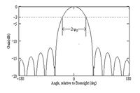
Antennas for DF have to meet different requirements from those for a radar or communication link, where an antenna with a narrow beam and high gain is usually an advantage. However, when carrying out direction finding, the bearing of the source may be unknown, so antennas with wide
The figure shows the normalized
Typically, the boresight gain of an antenna is related to the beam width.[26]: 257 For a rectangular horn, Gain ≈ 30000/BWh.BWv, where BWh and BWv are the horizontal and vertical antenna beamwidths, respectively, in degrees. For a circular aperture, with beamwidth BWc, it is Gain ≈ 30000/BWc2.
Two antenna types, popular for DF, are cavity-backed spirals and horn antennas.
-
 Antenna polar plot
 -
 Antenna log plot
 -
 Cavity backed spiral
 -
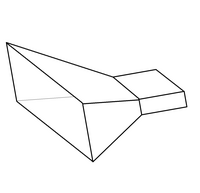 Pyramidal horn


Spiral antennas are capable of very wide bandwidths [26]: 252 [27] and have a nominal half-power beamwidth of about 70deg, making them very suitable for antenna arrays containing 4, 5 or 6 antennas.[18]: 41
For larger arrays, needing narrower
Microwave receivers
Early receivers
Early microwave receivers were usually simple "crystal-video" receivers,[31]: 169 [18]: 172 [32] which use a crystal detector followed by a video amplifier with a compressive characteristic to extend the dynamic range. Such a receiver was wideband but not very sensitive. However, this lack of sensitivity could be tolerated because of the "range advantage" enjoyed by the DF receiver (see below).
Klystron and TWT preamplifiers
The klystron and TWT are linear devices and so, in principle, could be used as receiver preamplifiers. However, the klystron was quite unsuitable as it was a narrow-band device and extremely noisy[21]: 392 and the TWT, although potentially more suitable,[21]: 548 has poor matching characteristics and large bulk, which made it unsuitable for multi-channel systems using a preamplifier per antenna. However, a system has been demonstrated, in which a single TWT preamplifier selectively selects signals from an antenna array.[33]
Transistor preamplifiers
Transistors suitable for microwave frequencies became available towards the end of the 1950s. The first of these was the
Range advantage
Source:[34]
The DF receiver enjoys a detection range advantage
In practice, the advantage is reduced by the ratio of antenna gains (typically they are 36 dB and 10 dB for the Radar and ESM, respectively) and the use of
The new demands on DF systems
The move to microwave frequencies meant a reappraisal of the requirements of a DF system.
In general, in order to cater for modern circumstances, a broadband microwave DF system is required to have high sensitivity and have 360° coverage in order to have the ability to detect single pulses (often called
DF by amplitude comparison
Amplitude comparison has been popular as a method for DF because systems are relatively simple to implement, have good sensitivity and, very importantly, a high probability of signal detection.[43]: 97 [18]: 207 Typically, an array of four, or more, squinted directional antennas is used to give 360 degree coverage.[44]: 155 [18]: 101 [45]: 5–8.7 [43]: 97 [46] DF by phase comparison methods can give better bearing accuracy,[45]: 5–8.9 but the processing is more complex. Systems using a single rotating dish antenna are more sensitive, small and relatively easy to implement, but have poor PoI.[42]
Usually, the signal amplitudes in two adjacent channels of the array are compared, to obtain the bearing of an incoming wavefront but, sometimes, three adjacent channels are used to give improved accuracy. Although the gains of the antennas and their amplifying chains have to be closely matched, careful design and construction and effective calibration procedures can compensate for shortfalls in the hardware. Overall bearing accuracies of 2° to 10° (rms) have been reported [45][47] using the method.
Two-channel DF


Two-channel DF, using two adjacent antennas of a circular array, is achieved by comparing the signal power of the largest signal with that of the second largest signal. The direction of an incoming signal, within the arc described by two antennas with a squint angle of Φ, may be obtained by comparing the relative powers of the signals received. When the signal is on the boresight of one of the antennas, the signal at the other antenna will be about 12 dB lower. When the signal direction is halfway between the two antennas, signal levels will be equal and approximately 3 dB lower than the boresight value. At other bearing angles, φ, some intermediate ratio of the signal levels will give the direction.
If the antenna main lobe patterns have a Gaussian characteristic, and the signal powers are described in logarithmic terms (e.g.
To give 360° coverage, antennas of a circular array are chosen, in pairs, according to the signal levels received at each antenna. If there are N antennas in the array, at angular spacing (squint angle) Φ, then Φ = 2π/N radians (= 360/N degrees).
Basic equations for two-port DF
If the main lobes of the antennas have a Gausian characteristic, then the output P1(φ), as a function of bearing angle φ, is given by[18]: 238
![{\displaystyle P_{1}(\phi )=G_{0}.\exp {\Bigr [}-A.{\Big (}{\frac {\phi }{\Psi _{0}}}{\Big )}^{2}{\Bigr ]}}](https://wikimedia.org/api/rest_v1/media/math/render/svg/5f15d7dd42215d4cc1c027bf5b8131d0aed564f8)
where
- G0 is the antenna boresight gain (i.e. when ø = 0),
- Ψ0 is one half the half-power beamwidth
- A = -\ln(0.5), so that P1(ø)/P10 = 0.5 when ø = Ψ0
- and angles are in radians.
The second antenna, squinted at Phi and with the same boresight gain G0 gives an output
![{\displaystyle P_{2}=G_{0}.\exp {\Bigr [}-A.{\Big (}{\frac {\Phi -\phi }{\Psi _{0}}}{\Big )}^{2}{\Bigr ]}}](https://wikimedia.org/api/rest_v1/media/math/render/svg/4bc00f945971d79d862beef86c331cda16c84758)
Comparing signal levels,
![{\displaystyle {\frac {P_{1}}{P_{2}}}={\frac {\exp {\big [}-A.(\phi /\Psi _{0})^{2}{\big ]}}{\exp {\Big [}-A{\big [}(\Phi -\phi )/\Psi _{0}{\big ]}^{2}{\Big ]}}}=\exp {\Big [}{\frac {A}{\Psi _{0}^{2}}}.(\Phi ^{2}-2\Phi \phi ){\Big ]}}](https://wikimedia.org/api/rest_v1/media/math/render/svg/2d96901e6bd34d6d62ba99c6ea643fe8c2b59a60)
The natural logarithm of the ratio is

Rearranging
![{\displaystyle \phi ={\frac {\Psi _{0}^{2}}{2A.\Phi }}.{\big [}\ln(P_{2})-\ln(P_{1}){\big ]}+{\frac {\Phi }{2}}}](https://wikimedia.org/api/rest_v1/media/math/render/svg/86d7f75574799ac307ce780b77f7aae1d52d33a6)
This shows the linear relationship between the output level difference, expressed logarithmically, and the bearing angle ø.
Natural logarithms can be converted to
![{\displaystyle \phi ={\frac {\Psi _{0}^{2}}{6.0202\Phi }}.{\big [}P_{2}(dB)-P_{1}(dB){\big ]}+{\frac {\Phi }{2}}}](https://wikimedia.org/api/rest_v1/media/math/render/svg/b247d0bdef7c7453e0a57108a6662c6e39cb78f9)
Three-channel DF


Improvements in bearing accuracy may be achieved if amplitude data from a third antenna are included in the bearing processing.[48][44]: 157
For three-channel DF, with three antennas squinted at angles Φ, the direction of the incoming signal is obtained by comparing the signal power of the channel containing the largest signal with the signal powers of the two adjacent channels, situated at each side of it.
For the antennas in a circular array, three antennas are selected according to the signal levels received, with the largest signal present at the central channel.
When the signal is on the boresight of Antenna 1 (φ = 0), the signal from the other two antennas will equal and about 12 dB lower. When the signal direction is halfway between two antennas (φ = 30°), their signal levels will be equal and approximately 3 dB lower than the boresight value, with the third signal now about 24 dB lower. At other bearing angles, ø, some intermediate ratios of the signal levels will give the direction.
Basic equations for three-port DF
For a signal incoming at a bearing ø, taken here to be to the right of boresight of Antenna 1:
Channel 1 output is
![{\displaystyle P_{1}=G_{T}.\exp {\Bigr [}-A.{\Big (}{\frac {\phi }{\Psi _{0}}}{\Big )}^{2}{\Bigr ]}}](https://wikimedia.org/api/rest_v1/media/math/render/svg/9cd6ef95366a8a132a862b8e6ddb8b1a993f8aea)
Channel 2 output is
![{\displaystyle P_{2}=G_{T}.\exp {\Bigr [}-A.{\Big (}{\frac {\Phi -\phi }{\Psi _{0}}}{\Big )}^{2}{\Bigr ]}}](https://wikimedia.org/api/rest_v1/media/math/render/svg/ed0e9099b9ee075ea7e910dad6b6c66baef9879d)
Channel 3 output is
![{\displaystyle P_{3}=G_{T}.\exp {\Bigr [}-A.{\Big (}{\frac {\Phi +\phi }{\Psi _{0}}}{\Big )}^{2}{\Bigr ]}}](https://wikimedia.org/api/rest_v1/media/math/render/svg/463e9864a50090bb2beb5f93397df4bbe6a67024)
where GT is the overall gain of each channel, including antenna boresight gain, and is assumed to be the same in all three channels. As before, in these equations, angles are in radians, Φ = 360/N degrees = 2 π/N radians and A = -ln(0.5).
As earlier, these can be expanded and combined to give:


Eliminating A/Ψ02 and rearranging

where Δ1,3 = \ln(P1) - ln(P3), Δ1,2 = \ln(P1) - \ln(P2) and Δ2,3 = \ln(P2) - \ln(P3),
The difference values here are in
The bearing value, obtained using this equation, is independent of the antenna beamwidth (= 2.Ψ0), so this value does not have to be known for accurate bearing results to be obtained. Also, there is a smoothing affect, for bearing values near to the boresight of the middle antenna, so there is no discontinuity in bearing values there, as an incoming signals moves from left to right (or vice versa) through boresight, as can occur with 2-channel processing.
Bearing uncertainty due to noise
Many of the causes of bearing error, such as mechanical imperfections in the antenna structure, poor gain matching of receiver gains, or non-ideal antenna gain patterns may be compensated by calibration procedures and corrective look-up tables, but
In general, a guide to bearing uncertainty is given by [45][51]>: 82 [31]: 91 [52]: 244
- degrees

for a signal at crossover, but where SNR0 is the signal-to-noise ratio that would apply at boresight.
To obtain more precise predictions at a given bearing, the actual S:N ratios of the signals of interest are used. (The results may be derived assuming that noise induced errors are approximated by relating differentials to uncorrelated noise).
For adjacent processing using, say, Channel 1 and Channel 2, the bearing uncertainty (angle noise), Δø (rms), is given below.[18][31]: 91 [53] In these results, square-law detection is assumed and the SNR figures are for signals at video (baseband), for the bearing angle φ.
- rads

where SNR1 and SNR2 are the video (base-band) signal-to-noise values for the channels for Antenna 1 and Antenna 2, when square-law detection is used.
In the case of 3-channel processing, an expression which is applicable when the S:N ratios in all three channels exceeds unity (when ln(1 + 1/SNR) ≈ 1/SNR is true in all three channels), is

where SNR1, SNR2 and SNR3 are the video signal-to-noise values for Channel 1, Channel 2, and Channel 3 respectively, for the bearing angle φ.
A typical DF system with six antennas

A schematic of a possible DF system,[18]: 101 employing six antennas,[54][55] is shown in the figure.
The signals received by the antennas are first amplified by a low-noise preamplifier before detection by detector-log-video-amplifiers (DLVAs).[56][57][58] The signal levels from the DLVAs are compared to determine the angle of arrival. By considering the signal levels on a logarithmic scale, as provided by the DLVAs, a large dynamic range is achieved [56]: 33 and, in addition, the direction finding calculations are simplified when the main lobes of antenna patterns have a Gaussian characteristic, as shown earlier.
A necessary part of the DF analysis is to identify the channel which contains the largest signal and this is achieved by means of a fast comparator circuit.[44] In addition to the DF process, other properties of the signal may be investigated, such as pulse duration, frequency, pulse repetition frequency (PRF) and modulation characteristics.[45] The comparator operation usually includes hysteresis, to avoid jitter in the selection process when the bearing of the incoming signal is such that two adjacent channels contain signals of similar amplitude.
Often, the wideband amplifiers are protected from local high power sources (as on a ship) by input limiters and/or filters. Similarly the amplifiers might contain notch filters to remove known, but unwanted, signals which could impairs the system's ability to process weaker signals. Some of these issues are covered in RF chain.
See also
- Amplitude monopulse
- AN/FLR-9, a cold war US Air Force HF direction finding system.
- AN/FRD-10, a cold war US Navy HF direction finding system.
- Battle of the Beams
- Electric beacon
- Geolocation
- Indoor positioning system
- MUSIC (algorithm)
- Phase interferometry
- Position fixing
- Radio determination
- Radio fix
- Radio location
- Real-time locating system
- TDOA
- VOR/DME
- Wullenweber
References
- ^ "Next Gen Implementation Plan 2013" (PDF). Archived from the original (PDF) on 2013-10-23.
- ^ a b c "Radar (Radio Direction Finding) – The Eyes of Fighter Command".
- ^ Yeang 2013, p. 187.
- ^ Baker 2013, p. 150.
- ^ Howeth 1963, p. 261.
- ^ Yeang 2013, p. 188.
- ^ "Broadcast Station Can Guide Flyer", April 1931, Popular Science
- ^ "Die Geschichte des Funkpeilens". www.seefunknetz.de. Retrieved 2023-08-11.
- ^ Bauer, Arthur O. (27 December 2004). "HF/DF An Allied Weapon against German U-boats 1939–1945" (PDF). Retrieved 2008-01-26. A paper on the technology and practice of the HF/DF systems used by the Royal Navy against U-boats in World War II
- ^ Gebhard, Louis A "Evolution of Naval Radio-Electronics and Contributions of the Naval Research Laboratory" (1979)
- ISBN 0-7509-3783-1.
- ^ Elliott (1972), p. 264
- ^ Keen, R (1947). Wireless Direction Finding (4th ed.). London, UK: Iliffe.
- ^
deRosa, L.A. (1979). "Direction Finding". In J.A. Biyd; D.B. Harris; D.D. King; H.W. Welch Jr. (eds.). Electronic Countermeasures. Los Altos, CA: Peninsula Publishing. ISBN 0-932146-00-7.
- ^ *J. Hereford & B. Edgerly (2000). "457 kHz Electromagnetism and the Future of Avalanche Transceivers" (PDF). International Snow Science Workshop (ISSW 2000). Archived from the original (PDF) on July 22, 2011.
- ISBN 978-1-905086-27-6.
- ^ Tsui J.B., "Microwave Receivers with Electronic Warfare Applications", Kreiber, 1992
- ^ a b c d e f g h i j Lipsky S.E., "Microwave Passive Direction Finding", Wiley 1987
- ^ Richardson D, "Techniques and Equipment of Electronic Warfare", Arco Publishing N.Y., 1985
- ^ a b c d e Gilmour jnr. A.S., "Microwave Tubes", Artech House, 1986
- ^ a b c Beck, A. H. W., "Thermionic Valves", Cambridge University Press, 1953
- ^ Baden Fuller A. J., "Microwaves"Pergamon Press, 1979
- ^ Hooijmans P., "Philip's tuner history". Find at http://maximus-randd.com/tv-tuner-history-pt1.html
- ^ a b c Gupta K.C., "Microwaves", New Age Intnl. Pub., 2012
- ^ Tutorial, "Advantages of Microwaves", Microwave Engineering Introduction article
- ^ a b Stutzman W.L. & Thiele G.A., "Antenna Theory and Design", 2nd Ed., Wiley 1998.
- ^ Morgan T.E., "Spiral Horns for ESM", IEE proc., Vol. 132, Pt. F., No. 4, July 1985, pp. 245 - 251
- ^ Milligan T.A., "Modern Antenna Design", 2nd Ed., Wiley 2005
- ^ a b Kingsley S. and Quegan S., "Understanding Radar Systems", McGraw -Hill 1992, SciTech Publishing, 1999
- ^ Clarricoats P.J.B and Olver A.D., "Corrugated horns for microwave antennas", Peter Perigrinus 1984
- ^ a b c Wiley R. G., Electronic Intelligence: The Interception of Radar Signals, Artech House, 1985
- ^ Lipkin H.J., "Crystal-Video Receivers", MIT Radiation Series Vol 23, Microwave Receivers, Chapter 19 pp.504-506. Find at: https://archive.org/details/MITRadiationLaboratorySeries23MicrowaveReceivers
- ^ Kiely D.G., "Advances in microwave direction finding", Proc. IEE, Vol. 113, No.11, Nov 1964, pp. 1967–1711
- ^ East P.W., "ESM Range Advantage", IEE Proceedings F - Communications, Radar and Signal Processing, Vol.132, No.4, Jul 1985, pp. 223 - 225
- ^ Davidson K., "Electronic Support Sensors". Find at: https://radar-engineer.com/files/Lecture_ES_Sensors.pdf
- ^ Connor F.R., "Antennas", Edward Arnold, 1972, p.8.
- ^ Woolier D.F., "System considerations for naval ESM", IEE Proc. Vol. 132, Pt. F, No. 4, July 1985.
- ^ Wise J.C., "A Perspective on EW Receiver Design", Tech. Report APA-TR-2009-1102, J.C. Wise and Associates, Nov. 2009, Find at:. https://ausairpower.net/APA-Maritime-ESM.html
- ^ Davidson K., "Low Probability of Intercept", find at: http://radar-engineer.com/files/Lecture_LPI_Radar.pdf
- ^ Stove A.G. Hume A.L. and Baker C.j., "Low probability of intercept radar strategies", IEE Proc. Sonar Navig., Vol. 151, No. 5, October 2004
- ^ Mills R.F. and Prescott G.E., "Detectability Models for Multiple Access Low-Probability-of-Intercept Networks", IEEE Trans on Aerospace and Electronic System, Vol.36, No.3, July 2000, pp> 848-858.
- ^ a b Hatcher B.R., "EW Acquisition Systems - probability of intercept and intercept times", Watkins-Johnson Tech-notes Vol. 3, No. 3, May/June 1976
- ^ a b Tsui J.B., "Microwave Receivers with Electronic Warfare Applications", Kreiber, Florida, 1992"
- ^ a b c East P.W., "Microwave System Design Tools with EW Applications", Artech House, 2nd Ed., 2008
- ^ a b c d e National Air Warfare Center, "Electronic Warfare and Radar Systems", NAWCWD TP 8347, 4th Ed., 2013. Find at: www.microwaves101.com/encyclopedias/ew-and-radar-handbook)
- ^ Ly P.Q.C, "Fast and Unabiguous Direction Finding for Digital Radar Intercept Receivers", Univ. of Adelaide, Dec. 2013, p. 16. Find at: https://digital.library.adelaide.edu.au/dspace/bitstream/2440/90332/4/02whole.pdf
- ^ Blake B. (ed.), "Manta", " Sceptre" and " Cutlass" ESM Systems, Jane's Radar and Electronic Warfare Systems, 1st Ed., Jane's Information Group, 1989, pp.344 -345
- ^ Stott G.F., "DF Algorithms for ESM", Military Microwaves '88 Conference Proceedings, London, July 1988, pp. 463 – 468
- ^ Connor F. R., Noise, Edward Arnold, London, 2nd ed. 1982, p. 44
- ^ Schwartz M., "Information Transmission, Modulation and Noise", McGraw-Hill, N.Y.,4th Ed., 1990, p.525
- ^ Al-Sharabi K.I.A. and Muhammad D.F., "Design of Wideband Radio Direction Finder Based on Amplitude Comparison", Al-Rafidain Engineering, Vol. 19, Oct 2011, pp.77-86 (Find at: www.iasj.net/iasj?func=fulltext&aid=26752 )
- ^ Martino A. De, "Introduction to Modern EW Systems", 2nd Ed., Artech House 2012
- ^ East P, "Microwave Intercept Receiver Sensitivity Estimation", Racal Defence Systems Report, 1998
- ^ Blake B. (ed.), " Cutlass ESM Equipment", Jane's Radar and Electronic Warfare Systems, 3rd Ed., Jane's Information Group, 1991, p. 406
- ^ Streetly M., "SPS-N 5000 ESM System", Jane's Radar and Electronic Warfare Systems, 10th Ed., Jane's Information Group, 1998, p. 396
- ^ a b MITEQ, "IF Signal Processing Components and Subsystems", Application Notes" pp. 33-51, (2010), Find at: https://nardamiteq.com/docs/MITEQ_IFsignal_c17.pdf
- ^ Pasternack, " Broadband Log Video Amplifiers". Find at: www.pasternack.com/pages/Featured_Products/broadband-log-video-amplifiers
- ^ American Microwave Corporation, DLVA Model: LVD-218-50. Find at: www.americanmic.com/catalog/detector-log-video-amplifiers-dlva/
Bibliography
- Baker, W. J. (2013). A History of the Marconi Company 1874-1965. Routledge. ISBN 9781134526079.
- Elliott, Peter (1972). "The Lend-Lease Captains". Warship International (3). International Naval Research Organization: 255.
- Appleyard, S.F.; Linford, R.S.; Yarwood, P.J. (1988). Marine Electronic Navigation (2nd ed.). Routledge & Kegan Paul. pp. 68–69. ISBN 0-7102-1271-2.
- M. Bondarenko and V.I. Slyusar. (August 2011). "Influence of jitter in ADC on precision of direction-finding by digital antenna arrays" (PDF). Radioelectronics and Communications Systems. 54 (8): 436–445. S2CID 110506568.
- Howeth, Linwood (1963). History of Communications-Electronics in the United States Navy. US Navy. pp. 261–265.
- Yeang, Chen-Pang (2013). Probing the Sky with Radio Waves. University of Chicago Press. ISBN 9780226015194.
- Radio Direction Finding Applications Literature (RDF Products)
- Doppler Systems Application Notes (Doppler Systems)