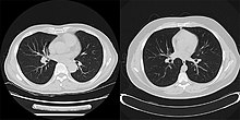
Iterative reconstruction

This article needs additional citations for verification. Please help improve this article by adding citations to reliable sources. Unsourced material may be challenged and removed. Find sources: "Iterative reconstruction" – news · newspapers · books · scholar · JSTOR (July 2007) (Learn how and when to remove this template message)

Iterative reconstruction refers to

techniques. For example, in

computed tomography

an image must be reconstructed from projections of an object. Here, iterative reconstruction techniques are usually a better, but computationally more expensive alternative to the common

filtered back projection

(FBP) method, which directly calculates the image in a single reconstruction step.[1] In recent research works, scientists have shown that extremely fast computations and massive parallelism is possible for iterative reconstruction, which makes iterative reconstruction practical for commercialization.^[2]

Basic concepts

The reconstruction of an image from the acquired data is an inverse problem. Often, it is not possible to exactly solve the inverse problem directly. In this case, a direct algorithm has to approximate the solution, which might cause visible reconstruction artifacts in the image. Iterative algorithms approach the correct solution using multiple iteration steps, which allows to obtain a better reconstruction at the cost of a higher computation time.

There are a large variety of algorithms, but each starts with an assumed image, computes projections from the image, compares the original projection data and updates the image based upon the difference between the calculated and the actual projections.

Algebraic reconstruction

The Algebraic Reconstruction Technique (ART) was the first iterative reconstruction technique used for

.

iterative Sparse Asymptotic Minimum Variance

The iterative Sparse Asymptotic Minimum Variance algorithm is an iterative, parameter-free superresolution tomographic reconstruction method inspired by compressed sensing, with applications in synthetic-aperture radar, computed tomography scan, and magnetic resonance imaging (MRI).

Statistical reconstruction

There are typically five components to statistical iterative image reconstruction algorithms, e.g.^[3]

1. An object model that expresses the unknown continuous-space function ${\displaystyle f(r)}$ that is to be reconstructed in terms of a finite series with unknown coefficients that must be estimated from the data.
2. A system model that relates the unknown object to the "ideal" measurements that would be recorded in the absence of measurement noise. Often this is a linear model of the form ${\displaystyle \mathbf {A} x+\epsilon }$, where ${\displaystyle \epsilon }$ represents the noise.
3. A
   Poisson statistics
   are closer to reality, it is more widely used.
4. A
   Markov random fields
   .
5. An algorithm, usually iterative, for minimizing the cost function, including some initial estimate of the image and some stopping criterion for terminating the iterations.

Learned Iterative Reconstruction

In learned iterative reconstruction, the updating algorithm is learned from training data using techniques from

Advantages

human heart. a) direct reconstruction b) iterative (nonlinear inverse) reconstruction^[6]

The advantages of the iterative approach include improved insensitivity to

are relatively poor.

Statistical, likelihood-based approaches: Statistical, likelihood-based iterative

are now the preferred method of reconstruction. Such algorithms compute estimates of the likely distribution of annihilation events that led to the measured data, based on statistical principle, often providing better noise profiles and resistance to the streak artifacts common with FBP. Since the density of radioactive tracer is a function in a function space, therefore of extremely high-dimensions, methods which regularize the maximum-likelihood solution turning it towards penalized or maximum a-posteriori methods can have significant advantages for low counts. Examples such as Ulf Grenander's Sieve estimator^[9][10] or Bayes penalty methods,

I.J. Good's roughness method^[13][14]

may yield superior performance to expectation-maximization-based methods which involve a Poisson likelihood function only.

As another example, it is considered superior when one does not have a large set of projections available, when the projections are not distributed uniformly in angle, or when the projections are sparse or missing at certain orientations. These scenarios may occur in

require the exclusion of some portions of the projection data.

In

to improve the reconstruction. For example, with iterative algorithms it is possible to reconstruct images from data acquired in a very short time as required for real-time MRI (rt-MRI).^[6]

In

Here is an example that illustrates the benefits of iterative image reconstruction for cardiac MRI.[21]

See also

• Tomographic reconstruction
• Positron Emission Tomography
• Tomogram
• Computed Tomography
• Magnetic Resonance Imaging
• Inverse problem
• Osem
• Deconvolution
• Inpainting
• Algebraic Reconstruction Technique
• iterative Sparse Asymptotic Minimum Variance

References

^{[1] [2]}

Wikimedia Commons has media related to Iterative reconstruction.

1. PMID 12368373
   .
2. ^ Grishentcev A. Jr (2012). "Effective compression of images on the basis of differential analysis" (PDF). Journal of Radio Electronics. 11: 1–42.