
Marine food web
| Part of a series of overviews on |
| Marine life |
|---|
 |
Compared to terrestrial environments, marine environments have
Because of this inversion, it is the
If phytoplankton dies before it is eaten, it descends through the
An ecosystem cannot be understood without knowledge of how its food web determines the flow of materials and energy. Phytoplankton autotrophically produces biomass by converting
Food chains and trophic levels
| marine food chain (typical) |
|---|
|
|
| ↓ |
| phytoplankton |
| ↓ |
| herbivorous zooplankton |
| ↓ |
| carnivorous zooplankton |
| ↓ |
|
|
| ↓ |
|
|
Food webs are built from food chains. All forms of life in the sea have the potential to become food for another life form. In the ocean, a food chain typically starts with energy from the sun powering phytoplankton, and follows a course such as:
phytoplankton → herbivorous zooplankton → carnivorous zooplankton → filter feeder → predatory vertebrate
In turn, the smaller herbivorous zooplankton are consumed by larger carnivorous zooplankters, such as larger predatory protozoa and


The fourth trophic level consists of predatory fish, marine mammals and seabirds that consume forage fish. Examples are swordfish, seals and gannets.
Apex predators, such as orcas, which can consume seals, and shortfin mako sharks, which can consume swordfish, make up a fifth trophic level. Baleen whales can consume zooplankton and krill directly, leading to a food chain with only three or four trophic levels.
In practice, trophic levels are not usually simple integers because the same consumer species often feeds across more than one trophic level.[8][9] For example a large marine vertebrate may eat smaller predatory fish but may also eat filter feeders; the stingray eats crustaceans, but the hammerhead eats both crustaceans and stingrays. Animals can also eat each other; the cod eats smaller cod as well as crayfish, and crayfish eat cod larvae. The feeding habits of a juvenile animal, and, as a consequence, its trophic level, can change as it grows up.
The fisheries scientist Daniel Pauly sets the values of trophic levels to one in primary producers and detritus, two in herbivores and detritivores (primary consumers), three in secondary consumers, and so on. The definition of the trophic level, TL, for any consumer species is[10]

where is the fractional trophic level of the prey j, and represents the fraction of j in the diet of i. In the case of marine ecosystems, the trophic level of most fish and other marine consumers takes value between 2.0 and 5.0. The upper value, 5.0, is unusual, even for large fish,[11] though it occurs in apex predators of marine mammals, such as polar bears and killer whales.[12] As a point of contrast, humans have a mean trophic level of about 2.21, about the same as a pig or an anchovy.[13][14]


By taxon
Primary producers

At the base of the ocean food web are single-celled algae and other plant-like organisms known as
Marine phytoplankton form the basis of the marine food web, account for approximately half of global carbon fixation and oxygen production by photosynthesis

Among the phytoplankton are members from a phylum of bacteria called
- Phytoplankton form the base of the ocean foodchain
-
 Phytoplankton
 -
 Dinoflagellate
 -
 Diatoms


In oceans, most
Thus, in ocean environments, the first bottom trophic level is occupied principally by
The most important groups of phytoplankton include the diatoms and dinoflagellates. Diatoms are especially important in oceans, where according to some estimates they contribute up to 45% of the total ocean's primary production.[23] Diatoms are usually microscopic, although some species can reach up to 2 millimetres in length.
Primary consumers

The second trophic level (
The
Other particularly important groups of zooplankton are the
- Zooplankton form a second level in the ocean food chain
-
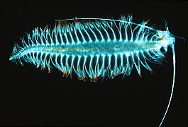 Segmented worm
 -
 Tiny shrimp-like crustaceans
 -
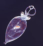 Juvenile planktonic squid


Together, phytoplankton and zooplankton make up most of the plankton in the sea. Plankton is the term applied to any small drifting organisms that float in the sea (Greek planktos = wanderer or drifter). By definition, organisms classified as plankton are unable to swim against ocean currents; they cannot resist the ambient current and control their position. In ocean environments, the first two trophic levels are occupied mainly by plankton. Plankton can be divided into producers and consumers. The producers are the phytoplankton (Greek phyton = plant) and the consumers, who eat the phytoplankton, are the zooplankton (Greek zoon = animal).
Higher order consumers

- Marine invertebrates
- Fish
- Forage fish: Forage fish occupy central positions in the ocean food webs. The organisms it eats are at a lower trophic level, and the organisms that eat it are at a higher trophic level. Forage fish occupy middle levels in the food web, serving as a dominant prey to higher level fish, seabirds and mammals.[29]
- Predator fish
- Ground fish
- Other marine vertebrates
In 2010 researchers found whales carry nutrients from the depths of the ocean back to the surface using a process they called the
-
 lunge from belowto feed on forage fish
 -
 plunge divefrom above to catch forage fish

,_Belmont_-_geograph.org.uk_-_529175.jpg)
-
 Whale pump nutrient cycle

Microorganisms

There has been increasing recognition in recent years that
In general,

- Viruses
A giant marine virus
Fungi
Parasitic
-
 Diagram of a mycoloop (fungus loop)
 -
 Roles of fungi in themarine carbon cycle by processing phytoplankton-derived organic matter


By habitat
Pelagic webs

For pelagic ecosystems, Legendre and Rassoulzadagan proposed in 1995 a continuum of trophic pathways with the herbivorous food-chain and microbial loop as food-web end members.[56] The classical linear food-chain end-member involves grazing by zooplankton on larger phytoplankton and subsequent predation on zooplankton by either larger zooplankton or another predator. In such a linear food-chain a predator can either lead to high phytoplankton biomass (in a system with phytoplankton, herbivore and a predator) or reduced phytoplankton biomass (in a system with four levels). Changes in predator abundance can, thus, lead to trophic cascades.[57] The microbial loop end-member involves not only phytoplankton, as basal resource, but also dissolved organic carbon.[58] Dissolved organic carbon is used by heterotrophic bacteria for growth are predated upon by larger zooplankton. Consequently, dissolved organic carbon is transformed, via a bacterial-microzooplankton loop, to zooplankton. These two end-member carbon processing pathways are connected at multiple levels. Small phytoplankton can be consumed directly by microzooplankton.[55]
As illustrated in the diagram on the right, dissolved organic carbon is produced in multiple ways and by various organisms, both by primary producers and consumers of organic carbon. DOC release by primary producers occurs passively by leakage and actively during unbalanced growth during nutrient limitation.
- Pelagic food web
-
![Pelagic food web and the biological pump. Links among the ocean's biological pump and pelagic food web and the ability to sample these components remotely from ships, satellites, and autonomous vehicles. Light blue waters are the euphotic zone, while the darker blue waters represent the twilight zone.[62]](//upload.wikimedia.org/wikipedia/commons/thumb/1/13/Export_Processes_in_the_Ocean_from_Remote_Sensing.jpg/627px-Export_Processes_in_the_Ocean_from_Remote_Sensing.jpg) Pelagic food web and theeuphotic zone, while the darker blue waters represent the twilight zone.[62]
Pelagic food web and theeuphotic zone, while the darker blue waters represent the twilight zone.[62]
![Pelagic food web and the biological pump. Links among the ocean's biological pump and pelagic food web and the ability to sample these components remotely from ships, satellites, and autonomous vehicles. Light blue waters are the euphotic zone, while the darker blue waters represent the twilight zone.[62]](/File:Export_Processes_in_the_Ocean_from_Remote_Sensing.jpg)
- Mesopelagic food web
-
![Impact of mesopelagic species on the global carbon budget.[63] DVM = diel vertical migration, NM = non-migration.](//upload.wikimedia.org/wikipedia/commons/thumb/5/54/Mesopelagic_species_impact_on_global_carbon_budget.png/652px-Mesopelagic_species_impact_on_global_carbon_budget.png) Impact of mesopelagic species on the global carbon budget.[63] DVM = diel vertical migration, NM = non-migration.
Impact of mesopelagic species on the global carbon budget.[63] DVM = diel vertical migration, NM = non-migration.
![Impact of mesopelagic species on the global carbon budget.[63] DVM = diel vertical migration, NM = non-migration.](/File:Mesopelagic_species_impact_on_global_carbon_budget.png)
-
![Mesopelagic bristlemouths may be the most abundant vertebrates on the planet, though little is known about them.[64]](//upload.wikimedia.org/wikipedia/commons/thumb/a/ac/Sigmops_bathyphilus1.jpg/368px-Sigmops_bathyphilus1.jpg) Mesopelagicbristlemouths may be the most abundant vertebrates on the planet, though little is known about them.[64]
Mesopelagicbristlemouths may be the most abundant vertebrates on the planet, though little is known about them.[64] -
 narcomedusanconsume the greatest diversity of mesopelagic prey
![Mesopelagic bristlemouths may be the most abundant vertebrates on the planet, though little is known about them.[64]](/File:Sigmops_bathyphilus1.jpg)


Scientists are starting to explore in more detail the largely unknown twilight zone of the
According to a 2017 study,
A 2020 study reported that by 2050 global warming could be spreading in the deep ocean seven times faster than it is now, even if emissions of greenhouse gases are cut. Warming in
- Fish in the twilight cast new light on ocean ecosystem The Conversation, 10 February 2014.
- An Ocean Mystery in the Trillions The New York Times, 29 June 2015.
- Mesopelagic fishes - Malaspina circumnavigation expedition of 2010.[69][70]

At the ocean surface
Ocean surface habitats sit at the interface between the ocean and the atmosphere. The
Unlike coloured algal blooms, surfactant-associated bacteria may not be visible in ocean colour imagery. Having the ability to detect these "invisible" surfactant-associated bacteria using
At the ocean floor
Ocean floor (
- Seeps and vents

Coastal webs
 | This article's images may require adjustment of the picture tutorial and the image placement policy for further information. (February 2023) |
Coastal waters include the waters in
Ecosystems, even those with seemingly distinct borders, rarely function independently of other adjacent systems.[80] Ecologists are increasingly recognizing the important effects that cross-ecosystem transport of energy and nutrients have on plant and animal populations and communities.[81][82] A well known example of this is how seabirds concentrate marine-derived nutrients on breeding islands in the form of feces (guano) which contains ~15–20% nitrogen (N), as well as 10% phosphorus.[83][84][85] These nutrients dramatically alter terrestrial ecosystem functioning and dynamics and can support increased primary and secondary productivity.[86][87] However, although many studies have demonstrated nitrogen enrichment of terrestrial components due to guano deposition across various taxonomic groups,[86][88][89][90] only a few have studied its retroaction on marine ecosystems and most of these studies were restricted to temperate regions and high nutrient waters.[83][91][92][93] In the tropics, coral reefs can be found adjacent to islands with large populations of breeding seabirds, and could be potentially affected by local nutrient enrichment due to the transport of seabird-derived nutrients in surrounding waters. Studies on the influence of guano on tropical marine ecosystems suggest nitrogen from guano enriches seawater and reef primary producers.[91][94][95]
Reef building corals have essential nitrogen needs and, thriving in nutrient-poor tropical waters[96] where nitrogen is a major limiting nutrient for primary productivity,[97] they have developed specific adaptations for conserving this element. Their establishment and maintenance are partly due to their symbiosis with unicellular dinoflagellates, Symbiodinium spp. (zooxanthellae), that can take up and retain dissolved inorganic nitrogen (ammonium and nitrate) from the surrounding waters.[98][99][100] These zooxanthellae can also recycle the animal wastes and subsequently transfer them back to the coral host as amino acids,[101] ammonium or urea.[102] Corals are also able to ingest nitrogen-rich sediment particles[103][104] and plankton.[105][106] Coastal eutrophication and excess nutrient supply can have strong impacts on corals, leading to a decrease in skeletal growth,[99][107][108][109][95]


In the diagram above on the right: (1) ammonification produces NH3 and NH4+ and (2) nitrification produces NO3− by NH4+ oxidation. (3) under the alkaline conditions, typical of the seabird feces, the NH3 is rapidly volatilised and transformed to NH4+, (4) which is transported out of the colony, and through wet-deposition exported to distant ecosystems, which are eutrophised. The phosphorus cycle is simpler and has reduced mobility. This element is found in a number of chemical forms in the seabird fecal material, but the most mobile and bioavailable is


DNA barcoding can be used to construct food web structures with better taxonomic resolution at the web nodes. This provides more specific species identification and greater clarity about exactly who eats whom. "DNA barcodes and DNA information may allow new approaches to the construction of larger interaction webs, and overcome some hurdles to achieving adequate sample size".[34]
A newly applied method for species identification is
- Microbial DNA barcoding
- Algae DNA barcoding
- Fish DNA barcoding
- DNA barcoding in diet assessment
- Kelp forests
- Byrnes, J.E., Reynolds, P.L. and Stachowicz, J.J. (2007) "Invasions and extinctions reshape coastal marine food webs". PLOS ONE, 2(3): e295.
Polar webs


Arctic and Antarctic marine systems have very different


- Arctic
The Arctic food web is complex. The loss of sea ice can ultimately affect the entire food web, from algae and plankton to fish to mammals. The impact of climate change on a particular species can ripple through a food web and affect a wide range of other organisms... Not only is the decline of sea ice impairing polar bear populations by reducing the extent of their primary habitat, it is also negatively impacting them via food web effects. Declines in the duration and extent of sea ice in the Arctic leads to declines in the abundance of ice algae, which thrive in nutrient-rich pockets in the ice. These algae are eaten by zooplankton, which are in turn eaten by Arctic cod, an important food source for many marine mammals, including seals. Seals are eaten by polar bears. Hence, declines in ice algae can contribute to declines in polar bear populations.[124]
In 2020 researchers reported that measurements over the last two decades on


- Antarctic
-
 Antarctic jellyfish Diplulmaris antarctica under the ice
 -
![Colonies of the alga Phaeocystis antarctica, an important phytoplankter of the Ross Sea that dominates early season blooms after the sea ice retreats and exports significant carbon.[129]](//upload.wikimedia.org/wikipedia/commons/thumb/a/a3/Phaeocystis.png/326px-Phaeocystis.png) Colonies of the alga Phaeocystis antarctica, an important phytoplankter of the Ross Sea that dominates early season blooms after the sea ice retreats and exports significant carbon.[129]
Colonies of the alga Phaeocystis antarctica, an important phytoplankter of the Ross Sea that dominates early season blooms after the sea ice retreats and exports significant carbon.[129] -
![The pennate diatom Fragilariopsis kerguelensis, found throughout the Antarctic Circumpolar Current, is a key driver of the global silicate pump.[130]](//upload.wikimedia.org/wikipedia/commons/thumb/4/4f/Fragilariopsis_kerguelensis.jpg/248px-Fragilariopsis_kerguelensis.jpg) Thepennate diatom Fragilariopsis kerguelensis, found throughout the Antarctic Circumpolar Current, is a key driver of the global silicate pump.[130]
Thepennate diatom Fragilariopsis kerguelensis, found throughout the Antarctic Circumpolar Current, is a key driver of the global silicate pump.[130] -
 A group ofkiller whales attempt to dislodge a crabeater seal on an ice floe
.jpg)
![Colonies of the alga Phaeocystis antarctica, an important phytoplankter of the Ross Sea that dominates early season blooms after the sea ice retreats and exports significant carbon.[129]](/File:Phaeocystis.png)
![The pennate diatom Fragilariopsis kerguelensis, found throughout the Antarctic Circumpolar Current, is a key driver of the global silicate pump.[130]](/File:Fragilariopsis_kerguelensis.jpg)


Polar microorganisms
In addition to the varied topographies and in spite of an extremely cold climate, polar aquatic regions are teeming with
Microorganisms are at the heart of Arctic and Antarctic food webs. These polar environments contain a diverse range of
Microbes, both
The polar regions are characterised by truncated food webs, and the role of viruses in ecosystem function is likely to be even greater than elsewhere in the marine food web. Their diversity is still relatively under-explored, and the way in which they affect polar communities is not well understood,[140] particularly in nutrient cycling.[138][148][149][46]
Foundation and keystone species
.jpg)
The concept of a foundation species was introduced in 1972 by Paul K. Dayton,[151] who applied it to certain members of marine invertebrate and algae communities. It was clear from studies in several locations that there were a small handful of species whose activities had a disproportionate effect on the rest of the marine community and they were therefore key to the resilience of the community. Dayton’s view was that focusing on foundation species would allow for a simplified approach to more rapidly understand how a community as a whole would react to disturbances, such as pollution, instead of attempting the extremely difficult task of tracking the responses of all community members simultaneously.
Foundation species are species that have a dominant role structuring an ecological community, shaping its environment and defining its ecosystem. Such ecosystems are often named after the foundation species, such as seagrass meadows, oyster beds, coral reefs, kelp forests and mangrove forests.[152] For example, the red mangrove is a common foundation species in mangrove forests. The mangrove’s root provides nursery grounds for young fish, such as snapper.[153] A foundation species can occupy any trophic level in a food web but tend to be a producer.[154]


The concept of the
Keystone species are species that have large effects, disproportionate to their numbers, within ecosystem food webs.
Topological position
Networks of trophic interactions can provide a lot of information about the functioning of marine ecosystems. Beyond feeding habits, three additional traits (mobility, size, and habitat) of various organisms can complement this trophic view.[162]

In order to sustain the proper functioning of ecosystems, there is a need to better understand the simple question asked by Lawton in 1994: What do species do in ecosystems?[163] Since ecological roles and food web positions are not independent,[164] the question of what kind of species occupy various of network positions needs to be asked.[162] Since the very first attempts to identify keystone species,[165][166] there has been an interest in their place in food webs.[167][168] First they were suggested to have been top predators, then also plants, herbivores, and parasites.[169][170] For both community ecology and conservation biology, it would be useful to know where are they in complex trophic networks.[162]
An example of this kind of network analysis is shown in the diagram, based on data from a marine food web.[171] It shows relationships between the topological positions of web nodes and the mobility values of the organism's involved. The web nodes are shape-coded according to their mobility, and colour-coded using indices which emphasise (A) bottom-up groups (sessile and drifters), and (B) groups at the top of the food web.[162]
The relative importance of organisms varies with time and space, and looking at large databases may provide general insights into the problem. If different kinds of organisms occupy different types of network positions, then adjusting for this in food web modelling will result in more reliable predictions. Comparisons of
Cryptic interactions
Cryptic interactions, interactions which are "hidden in plain sight", occur throughout the marine planktonic foodweb but are currently largely overlooked by established methods, which mean large‐scale data collection for these interactions is limited. Despite this, current evidence suggests some of these interactions may have perceptible impacts on foodweb dynamics and model results. Incorporation of cryptic interactions into models is especially important for those interactions involving the transport of nutrients or energy.[177]
The diagram illustrates the material fluxes, populations, and molecular pools that are impacted by five cryptic interactions:
Simplifications such as "zooplankton consume phytoplankton", "phytoplankton take up inorganic nutrients", "gross primary production determines the amount of carbon available to the food web", etc. have helped scientists explain and model general interactions in the aquatic environment. Traditional methods have focused on quantifying and qualifying these generalisations, but rapid advancements in genomics, sensor detection limits, experimental methods, and other technologies in recent years have shown that generalisation of interactions within the plankton community may be too simple. These enhancements in technology have exposed a number of interactions which appear as cryptic because bulk sampling efforts and experimental methods are biased against them.[177]
Complexity and stability

In 1927, Charles Elton published an influential synthesis on the use of food webs, which resulted in them becoming a central concept in ecology.[182] In 1966, interest in food webs increased after Robert Paine's experimental and descriptive study of intertidal shores, suggesting that food web complexity was key to maintaining species diversity and ecological stability.[183] Many theoretical ecologists, including Robert May and Stuart Pimm, were prompted by this discovery and others to examine the mathematical properties of food webs. According to their analyses, complex food webs should be less stable than simple food webs.[184]: 75–77 [185]: 64 The apparent paradox between the complexity of food webs observed in nature and the mathematical fragility of food web models is currently an area of intensive study and debate. The paradox may be due partially to conceptual differences between persistence of a food web and equilibrial stability of a food web.[184][185]
A trophic cascade can occur in a food web if a trophic level in the web is suppressed.
For example, a top-down cascade can occur if predators are effective enough in predation to reduce the abundance, or alter the behavior, of their
In a bottom-up cascade, the population of primary producers will always control the increase/decrease of the energy in the higher trophic levels. Primary producers are plants, phytoplankton and zooplankton that require photosynthesis. Although light is important, primary producer populations are altered by the amount of nutrients in the system. This food web relies on the availability and limitation of resources. All populations will experience growth if there is initially a large amount of nutrients.[189][190]
Terrestrial comparisons
.jpg)
.jpg)
Marine environments can have inversions in their biomass pyramids. In particular, the biomass of consumers (copepods, krill, shrimp, forage fish) is generally larger than the biomass of primary producers. This happens because the ocean's primary producers are mostly tiny phytoplankton which have
Examples: The bristlecone pine can live for thousands of years, and has a very low production/biomass ratio. The cyanobacterium Prochlorococcus lives for about 24 hours, and has a very high production/biomass ratio.
In oceans, most
| Ecosystem | Net primary productivity ( Gt/y )
|
Total plant biomass (Gt) | Turnover time (y) |
|---|---|---|---|
| Marine | 45–55 | 1–2 | 0.02–0.06 |
| Terrestrial | 55–70 | 600–1000 | 9–20 |

Aquatic producers, such as planktonic algae or aquatic plants, lack the large accumulation of
Most
.jpeg)
Anthropogenic effects

- Overfishing
- Acidification
Pteropods and brittle stars together form the base of the Arctic food webs and both are seriously damaged by acidification. Pteropods shells dissolve with increasing acidification and brittle stars lose muscle mass when re-growing appendages.[200] Additionally the brittle star's eggs die within a few days when exposed to expected conditions resulting from Arctic acidification.[201] Acidification threatens to destroy Arctic food webs from the base up. Arctic waters are changing rapidly and are advanced in the process of becoming undersaturated with aragonite.[202] Arctic food webs are considered simple, meaning there are few steps in the food chain from small organisms to larger predators. For example, pteropods are "a key prey item of a number of higher predators – larger plankton, fish, seabirds, whales".[203]
- Climate change
Ecosystems in the ocean are more sensitive to climate change than anywhere else on Earth. This is due to warmer temperatures and ocean acidification. With the ocean temperatures increasing, it is predicted that fish species will move from their known ranges and locate new areas. During this change, the numbers within each species will drop significantly. Currently there are many relationships between predators and prey, where they rely on one another to survive.[204] With a shift in where species will be located, the predator-prey relationships/interactions will be greatly impacted. Studies are still being done to understand how these changes will affect the food-web dynamics.
Using modeling, scientists are able to analyze the trophic interactions that certain species thrive in and due to other species also found in these areas. Through recent models, it is seen that many of the larger marine species will end up shifting their ranges at a slower pace than climate change suggests. This would impact the predator-prey relationship even more. As the smaller species and organisms are more likely to be influenced from the oceans warming and moving sooner than the larger mammals.[204] These predators are seen to stay longer in their historical ranges before moving because of the movement of the smaller species moving. With “new” species entering the space of the larger mammals, the ecology changes and more prey for them to feed upon.[204] The smaller species would end up having a smaller range, whereas the larger mammals would have extended their range. The shifting dynamics will have great effects on all species within the ocean and will result in many more changes impacting our entire ecosystem. With the movement in where predators can find prey within the ocean, will also impact the fisheries industry.[205] Where fishermen currently know where certain fish species occupy, as the shift occurs it will be more difficult to figure out where they are spending their time, costing them more money as they may have to travel further.[206] As a result this could impact the current fishing regulations set up for certain areas with the movement of these fish populations.
.png)
Through a survey conducted at Princeton University, researchers found that the marine species are consistently keeping pace with “climate velocity” or speed and direction in which it is moving. Looking at data from 1968 to 2011, it was found that 70 per cent of the shifts in animals’ depths and 74 per cent of changes in latitude correlated with regional-scale fluctuations in ocean temperature.[209] These movements are causing species to move between 4.5 and 40 miles per decade further away from the equator. With the help of models, regions can predict where the species may end up. Models will have to adapt to the changes as more is learned about how climate is affecting species.
"Our results show how future climate change can potentially weaken marine food webs through reduced energy flow to higher trophic levels and a shift towards a more detritus-based system, leading to food web simplification and altered producer–consumer dynamics, both of which have important implications for the structuring of benthic communities."[210][211]
"...increased temperatures reduce the vital flow of energy from the primary food producers at the bottom (e.g. algae), to intermediate consumers (herbivores), to predators at the top of marine food webs. Such disturbances in energy transfer can potentially lead to a decrease in food availability for top predators, which in turn, can lead to negative impacts for many marine species within these food webs... "Whilst climate change increased the productivity of plants, this was mainly due to an expansion of cyanobacteria (small blue-green algae)," said Mr Ullah. "This increased primary productivity does not support food webs, however, because these cyanobacteria are largely unpalatable and they are not consumed by herbivores. Understanding how ecosystems function under the effects of global warming is a challenge in ecological research. Most research on ocean warming involves simplified, short-term experiments based on only one or a few species."[211]


See also
References
- ^ U S Department of Energy (2008) Carbon Cycling and Biosequestration page 81, Workshop report DOE/SC-108, U.S. Department of Energy Office of Science.
- ^ Campbell, Mike (22 June 2011). "The role of marine plankton in sequestration of carbon". EarthTimes. Retrieved 22 August 2014.
- ^ Why should we care about the ocean? NOAA: National Ocean Service. Updated: 7 January 2020. Retrieved 1 March 2020.
- .
- .
- ISBN 9780199775057.
- Odum, W. E.; Heald, E. J. (1975) "The detritus-based food web of an estuarine mangrove community". Pages 265–286 in L. E. Cronin, ed. Estuarine research. Vol. 1. Academic Press, New York.
- S2CID 4161183.
- ^ Pauly, D.; Palomares, M. L. (2005). "Fishing down marine food webs: it is far more pervasive than we thought" (PDF). Bulletin of Marine Science. 76 (2): 197–211. Archived from the original (PDF) on 14 May 2013.
- .
- .
- ^ Researchers calculate human trophic level for first time Phys.org . 3 December 2013.
- .
- ^ a b Chlorophyll NASA Earth Observatory. Accessed 30 November 2019.
- PMID 30319587.
- PMID 9657713.
- S2CID 54551421.
- PMID 18159947.
- ^ Nemiroff, R.; Bonnell, J., eds. (27 September 2006). "Earth from Saturn". Astronomy Picture of the Day. NASA.
- PMID 10066832.
- ^ "The Most Important Microbe You've Never Heard Of". npr.org.
- .
- ISBN 978-1-4020-8239-9.
- Carl von Ossietzky University of Oldenburg
- ^
- ^ doi:10.1038/531432a
- National Public Radio, 7 April 2016.
- PMID 20949007. e13255.
- ^ Brown, Joshua E. (12 October 2010). "Whale poop pumps up ocean health". Science Daily. Retrieved 18 August 2014.
- doi:10.1128/mSystems.00150-17..
 Modified text was copied from this source, which is available under a Creative Commons Attribution 4.0 International License
 - ISBN 978-1-904455-87-5.
- ^ .
- JSTOR 1313569.
- ^ Weinbauer, Markus G., et al. "Synergistic and antagonistic effects of viral lysis and protistan grazing on bacterial biomass, production and diversity." Environmental Microbiology 9.3 (2007): 777-788.
- ^ Robinson, Carol, and Nagappa Ramaiah. "Microbial heterotrophic metabolic rates constrain the microbial carbon pump." The American Association for the Advancement of Science, 2011.
- .
- doi:10.1007/978-3-319-93284-2_5.. Modified text was copied from this source, which is available under a Creative Commons Attribution 4.0 International License
- .
- doi:10.1371/journal.ppat.1007592.. Modified text was copied from this source, which is available under a Creative Commons Attribution 4.0 International License
- ^ S2CID 4658457.
- ^ PMID 29057790.
- S2CID 4271861.
- PMID 26200428.
- ^ PMID 30813316.. Modified text was copied from this source, which is available under a Creative Commons Attribution 4.0 International License
- PMID 20974979.
- PMID 20974979.
- S2CID 30191542.
- S2CID 206530677.
- S2CID 4458402.
- doi:10.3389/fmicb.2014.00166.. Modified text was copied from this source, which is available under a Creative Commons Attribution 3.0 International License
- doi:10.1128/mBio.01189-18.. Modified text was copied from this source, which is available under a Creative Commons Attribution 4.0 International License
- .
- ^ S2CID 104330175.. Modified text was copied from this source, which is available under a Creative Commons Attribution 4.0 International License
- ^ Legendre L, Rassoulzadegan F (1995) "Plankton and nutrient dynamics in marine waters". Ophelia, 41:153–172.
- ^ Pace ML, Cole JJ, Carpenter SR, Kitchell JF (1999) "Trophic cascades revealed in diverse ecosystems". Trends Ecol Evol, 14: 483–488.
- ^ Azam F, Fenchel T, Field JG, Gray JS, Meyer-Reil LA, Thingstad F (1983) "The ecological role of water-column microbes in the sea". Mar Ecol-Prog Ser, 10: 257–263.
- ^ Anderson TR and LeB Williams PJ (1998) "Modelling the seasonal cycle of dissolved organic carbon at station E1 in the English channel". Estuar Coast Shelf Sci, 46: 93–109.
- ^ Van den Meersche K, Middelburg JJ, Soetaert K, van Rijswijk P, Boschker HTS, Heip CHR (2004) "Carbon–nitrogen coupling and algal–bacterial interactions during an experimental bloom: modeling a 13C tracer experiment". Limnol Oceanogr, 49: 862–878.
- ^ Suttle CA (2005) "Viruses in the sea". Nature, 437: 356–361.
- doi:10.3389/fmars.2016.00022.. Modified text was copied from this source, which is available under a Creative Commons Attribution 4.0 International License
- .
- ^ .
- ^ doi:10.1098/rspb.2017.2116.. Modified text was copied from this source, which is available under a Creative Commons Attribution 4.0 International License
- .
- ^ Climate change in deep oceans could be seven times faster by middle of century, report says The Guardian, 25 May 2020.
- .
- ^ Fish biomass in the ocean is 10 times higher than estimated EurekAlert, 7 February 2014.
- .
- ^ doi:10.1038/srep19123.. Modified text was copied from this source, which is available under a Creative Commons Attribution 4.0 International License
- .
- .
- .
- .
- .
- ^ doi:10.1038/s41467-017-02446-8. Modified text was copied from this source, which is available under a Creative Commons Attribution 4.0 International License.
- .
- S2CID 84701185.
- .
- ^ PMID 23593452.
- .
- PMID 18837063.
- ^ PMID 22723945.
- ISBN 9780199735693.
- S2CID 6021420.
- S2CID 12110520.
- PMID 26504209.
- ^ S2CID 87850538.
- .
- S2CID 83734364.
- .
- ^ S2CID 6539261.. Modified text was copied from this source, which is available under a Creative Commons Attribution 4.0 International License
- ISBN 9781351092777.
- PMID 21232343.
- JSTOR 1312147.
- ^ S2CID 85085823.
- ^ Muscatine, L. (1990) "The role of symbiotic algae in carbon and energy flux in reef corals", Ecosystem World, 25: 75–87.
- S2CID 25973061.
- PMID 21676806.
- S2CID 13212636.
- S2CID 84698653.
- .
- S2CID 44869188.
- S2CID 83654833.
- .
- .
- ISBN 9783319967769
- ^ Heymans, J.J., Coll, M., Libralato, S., Morissette, L. and Christensen, V. (2014). "Global patterns in ecological indicators of marine food webs: a modelling approach". PLOS ONE, 9(4). doi:10.1371/journal.pone.0095845.
- ^ Pranovi, F., Libralato, S., Raicevich, S., Granzotto, A., Pastres, R. and Giovanardi, O. (2003). "Mechanical clam dredging in Venice lagoon: ecosystem effects evaluated with a trophic mass-balance model". Marine Biology, 143(2): 393–403. doi:10.1007/s00227-003-1072-1.
- ^ US Geological Survey (USGS). "Chapter 14: Changes in Food and Habitats of Waterbirds." Figure 14.1. Synthesis of U.S. Geological Survey Science for the Chesapeake Bay Ecosystem and Implications for Environmental Management. USGS Circular 1316.
 This article incorporates text from this source, which is in the public domain.
- ^ Perry, M.C., Osenton, P.C., Wells-Berlin, A.M., and Kidwell, D.M., 2005, Food selection among Atlantic Coast sea ducks in relation to historic food habits, [abs.] in Perry, M.C., Second North American Sea Duck Conference, November 7–11, 2005, Annapolis, Maryland, Program and Abstracts, USGS Patuxent Wildlife Research Center, Maryland, 123 p. (p. 105).
- .
- doi:10.1371/journal.pone.0022591.. Modified text was copied from this source, which is available under a Creative Commons Attribution 4.0 International License
- .
- ISSN 2296-7745.. Modified text was copied from this source, which is available under a Creative Commons Attribution 4.0 International License
- ISBN 9783319319834
- ISBN 9780511763175
- ISBN 9780521015004
- PMID 27928038.
- ^ Climate Impacts on Ecosystems: Food Web Disruptions EPA. Accessed 11 February 2020. This article incorporates text from this source, which is in the public domain.
- ^ "A 'regime shift' is happening in the Arctic Ocean, scientists say". phys.org. Retrieved 16 August 2020.
- S2CID 220433818. Retrieved 16 August 2020.
- S2CID 216033140.. Modified text was copied from this source, which is available under a Creative Commons Attribution 4.0 International License
- S2CID 92529531.
- PMID 25473469.
- PMID 31628346... Modified text was copied from this source, which is available under a Creative Commons Attribution 4.0 International License
- ^ PMID 30225167.
- hdl:11336/39918.
- PMID 24832507.
- ^
- Azam, F.; Fenchel, T.; Field, J. G.; Gray, J. S.; Meyer-Reil, L. A.; Thingstad, F. (1983). "The Ecological Role of Water-Column Microbes in the Sea". Marine Ecology Progress Series. 10 (3): 257–263. JSTOR 24814647.
- Fenchel, Tom (2008). "The microbial loop – 25 years later". Journal of Experimental Marine Biology and Ecology. 366 (1–2): 99–103. .
- Azam, F.; Fenchel, T.; Field, J. G.; Gray, J. S.; Meyer-Reil, L. A.; Thingstad, F. (1983). "The Ecological Role of Water-Column Microbes in the Sea". Marine Ecology Progress Series. 10 (3): 257–263.
- ^ S2CID 20798336.
- PMC 4009764.
- ^ S2CID 33598792.
- S2CID 23089203.
- ^ PMID 21130655.
- ^ PMID 22000675.
- ^ PMID 23045668.
- ISSN 0091-7613.
- PMID 26069354.
- S2CID 129578736.
- ^ Adie, R.J. (1962) "The geology of Antarctica". In" Antarctic Research: The Matthew Fontaine Maury Memorial Symposium, John Wiley & Sons.
- .
- S2CID 32607904.
- S2CID 2927907.
- doi:10.1002/ecy.2987.
- ^ Dayton, P. K. 1972. Toward an understanding of community resilience and the potential effects of enrichments to the benthos at McMurdo Sound, Antarctica. pp. 81–96 in Proceedings of the Colloquium on Conservation Problems Allen Press, Lawrence, Kansas.
- ^ Giant kelp gives Southern California marine ecosystems a strong foundation, National Science Foundation, 4 February 2020.
- .
- hdl:11603/29165.
- S2CID 83780992.
- ^ "Keystone Species Hypothesis". University of Washington. Archived from the original on 10 January 2011. Retrieved 3 February 2011.
- S2CID 85265656.
- .
- ^ Davic, Robert D. (2003). "Linking Keystone Species and Functional Groups: A New Operational Definition of the Keystone Species Concept". Conservation Ecology. Archived from the original on 26 August 2003. Retrieved 3 February 2011.
- S2CID 84866250.
- JSTOR 1313259.
- ^ doi:10.3389/fmars.2021.636042.. Modified text was copied from this source, which is available under a Creative Commons Attribution 4.0 International License
- JSTOR 3545824.
- PMID 12468282.
- S2CID 38675566.
- JSTOR 1936888.
- JSTOR 1312122.
- JSTOR 1312990.
- ISBN 978-3-540-58103-1.
- PMID 21238094.
- .
- .
- .
- .
- .
- S2CID 90319704.
- ^ doi:10.1002/lol2.10084.. Modified text was copied from this source, which is available under a Creative Commons Attribution 4.0 International License
- ^ .
- .
- .
- ISBN 978-0-470-45546-3.
- ^ Elton CS (1927) Animal Ecology. Republished 2001. University of Chicago Press.
- S2CID 85265656.
- ^ ISBN 978-0-691-08861-7.
- ^ ISBN 978-0-226-66832-1.
- PMID 29651152.
- ^ Megrey, Bernard and Werner, Francisco. "Evaluating the Role of Topdown vs. Bottom-up Ecosystem Regulation from a Modeling Perspective" (PDF).
{{cite web}}: CS1 maint: multiple names: authors list (link) - S2CID 45088691.
- S2CID 46996957.
- PMID 28167770.
- ^ "Oldlist". Rocky Mountain Tree Ring Research. Retrieved 8 January 2013.
- ISBN 9780127447605.
- ^ PMID 9657713.
- .
- ISBN 978-1-4200-5544-3.
- ISBN 978-0-534-42066-6. Archived from the originalon 20 August 2011.
- doi:10.1016/j.ecolmodel.2009.03.005. Archived from the original(PDF) on 7 October 2011.
- PMID 17740399.
- ^ "Effects of Ocean Acidification on Marine Species & Ecosystems". Report. OCEANA. Archived from the original on 25 December 2014. Retrieved 13 October 2013.
- ^ "Comprehensive study of Arctic Ocean acidification". Study. CICERO. Archived from the original on 10 December 2013. Retrieved 14 November 2013.
- ^ Lischka, S.; Büdenbender J.; Boxhammer T.; Riebesell U. (15 April 2011). "Impact of ocean acidification and elevated temperatures on early juveniles of the polar shelled pteropod Limacina helicina : mortality, shell degradation, and shell growth" (PDF). Report. Biogeosciences. pp. 919–932. Retrieved 14 November 2013.
- ^ "Antarctic marine wildlife is under threat, study finds". BBC Nature. Retrieved 13 October 2013.
- ^ a b c Tekwa, E. W., J.R. Watson., M. L. Pinsky. “Body Size and Food–Web Interactions Mediate Species Range Shifts under Warming.” Proceedings of the Royal Society B: Biological Sciences, vol. 289, no. 1972, 2022, https://doi.org/10.1098/rspb.2021.2755.
- ^ Chapman, Eric J., C.J. Byron., R. Lasley-Rasher., C. Lipsky., J.R. Stevens., R. Peters. “Effects of Climate Change on Coastal Ecosystem Food Webs: Implications for Aquaculture.” Marine Environmental Research, vol. 162, 2020, p. 105103., https://doi.org/10.1016/j.marenvres.2020.105103
- ^ “Climate Change Impacts on the Ocean and Marine Resources.” EPA, Environmental Protection Agency, https://www.epa.gov/climateimpacts/climate-change-impacts-ocean-and-marine-resources
- ^ “Climate Change Indicators: Marine Species Distribution.” EPA, Environmental Protection Agency, https://www.epa.gov/climate-indicators/climate-change-indicators-marine-species-distribution#ref4.
- ^ NOAA (National Oceanic and Atmospheric Administration) and Rutgers University. 2021. OceanAdapt. Accessed January 2021 https://oceanadapt.rutgers.edu
- ^ Pinsky, Malin L., B. Worm., M.J. Forgarty., J.L. Sarmiento., S.A. Levin . “Marine Taxa Track Local Climate Velocities.” Science, vol. 341, no. 6151, 2013, pp. 1239–1242., https://doi.org/10.1126/science.1239352
- ^ a b Climate change drives collapse in marine food webs ScienceDaily. 9 January 2018.
- ^ IUCN (2018) The IUCN Red List of Threatened Species: Version 2018-1