Multigrid method

In

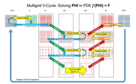
There are many variations of multigrid algorithms, but the common features are that a hierarchy of discretizations (grids) is considered. The important steps are:^[5][6]

• Smoothing – reducing high frequency errors, for example using a few iterations of the Gauss–Seidel method.
• Residual Computation – computing residual error after the smoothing operation(s).
• Restriction – downsampling the residual error to a coarser grid.
• Interpolation or prolongation – interpolating a correction computed on a coarser grid into a finer grid.
• Correction – Adding prolongated coarser grid solution onto the finer grid.

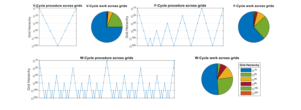
There are many choices of multigrid methods with varying trade-offs between speed of solving a single iteration and the rate of convergence with said iteration. The 3 main types are V-Cycle, F-Cycle, and W-Cycle. These differ in which and how many coarse-grain cycles are performed per fine iteration. The V-Cycle algorithm executes one coarse-grain V-Cycle. F-Cycle does a coarse-grain V-Cycle followed by a coarse-grain F-Cycle, while each W-Cycle performs two coarse-grain W-Cycles per iteration. For a discrete 2D problem, F-Cycle takes 83% more time to compute than a V-Cycle iteration while a W-Cycle iteration takes 125% more. If the problem is set up in a 3D domain, then a F-Cycle iteration and a W-Cycle iteration take about 64% and 75% more time respectively than a V-Cycle iteration ignoring overheads. Typically, W-Cycle produces similar convergence to F-Cycle. However, in cases of convection-diffusion problems with high Péclet numbers, W-Cycle can show superiority in its rate of convergence per iteration over F-Cycle. The choice of smoothing operators are extremely diverse as they include Krylov subspace methods and can be preconditioned.

Any geometric multigrid cycle iteration is performed on a hierarchy of grids and hence it can be coded using recursion. Since the function calls itself with smaller sized (coarser) parameters, the coarsest grid is where the recursion stops. In cases where the system has a high condition number, the correction procedure is modified such that only a fraction of the prolongated coarser grid solution is added onto the finer grid.

function phi = V_Cycle(phi,f,h)
    % Recursive V-Cycle Multigrid for solving the Poisson equation (\nabla^2 phi = f) on a uniform grid of spacing h

    % Pre-Smoothing
    phi = smoothing(phi,f,h);

    % Compute Residual Errors
    r = residual(phi,f,h);

    % Restriction
    rhs = restriction(r);

    eps = zeros(size(rhs));

    % stop recursion at smallest grid size, otherwise continue recursion
    if smallest_grid_size_is_achieved
        eps = coarse_level_solve(eps,rhs,2*h);
    else
        eps = V_Cycle(eps,rhs,2*h);
    end

    % Prolongation and Correction
    phi = phi + prolongation(eps);

    % Post-Smoothing
    phi = smoothing(phi,f,h);
end

function phi = F_Cycle(phi,f,h)
    % Recursive F-cycle multigrid for solving the Poisson equation (\nabla^2 phi = f) on a uniform grid of spacing h

    % Pre-smoothing
    phi = smoothing(phi,f,h);

    % Compute Residual Errors
    r = residual(phi,f,h);

    % Restriction
    rhs = restriction(r);

    eps = zeros(size(rhs));

    % stop recursion at smallest grid size, otherwise continue recursion
    if smallest_grid_size_is_achieved
        eps = coarse_level_solve(eps,rhs,2*h);
    else
        eps = F_Cycle(eps,rhs,2*h);
    end

    % Prolongation and Correction
    phi = phi + prolongation(eps);

    % Re-smoothing
    phi = smoothing(phi,f,h);

    % Compute residual errors
    r = residual(phi,f,h);

    % Restriction
    rhs = restriction(r);

    % stop recursion at smallest grid size, otherwise continue recursion
    if smallest_grid_size_is_achieved
        eps = coarse_level_solve(eps,rhs,2*h);
    else
        eps = V_Cycle(eps,rhs,2*h);
    end

    % Prolongation and Correction
    phi = phi + prolongation(eps);

    % Post-smoothing
    phi = smoothing(phi,f,h);
end

function phi = W_cycle(phi,f,h)
    % Recursive W-cycle multigrid for solving the Poisson equation (\nabla^2 phi = f) on a uniform grid of spacing h

    % Pre-smoothing
    phi = smoothing(phi,f,h);

    % Compute Residual Errors
    r = residual(phi,f,h);

    % Restriction
    rhs = restriction(r);

    eps = zeros(size(rhs));

    % stop recursion at smallest grid size, otherwise continue recursion
    if smallest_grid_size_is_achieved
        eps = coarse_level_solve(eps,rhs,2*h);
    else
        eps = W_cycle(eps,rhs,2*h);
    end

    % Prolongation and correction
    phi = phi + prolongation(eps);

    % Re-smoothing
    phi = smoothing(phi,f,h);

    % Compute residual errors
    r = residual(phi,f,h);

    % Restriction
    rhs = restriction(r);

    % stop recursion at smallest grid size, otherwise continue recursion
    if smallest_grid_size_is_achieved
        eps = coarse_level_solve(eps,rhs,2*h);
    else
        eps = W_cycle(eps,rhs,2*h);
    end

    % Prolongation and correction
    phi = phi + prolongation(eps);

    % Post-smoothing
    phi = smoothing(phi,f,h);
end

Computational cost ^{[citation needed]}

This approach has the advantage over other methods that it often scales linearly with the number of discrete nodes used. In other words, it can solve these problems to a given accuracy in a number of operations that is proportional to the number of unknowns.

Assume that one has a differential equation which can be solved approximately (with a given accuracy) on a grid ${\displaystyle i}$ with a given grid point density ${\displaystyle N_{i}}$. Assume furthermore that a solution on any grid ${\displaystyle N_{i}}$ may be obtained with a given effort ${\displaystyle W_{i}=\rho KN_{i}}$ from a solution on a coarser grid ${\displaystyle i+1}$. Here, ${\displaystyle \rho =N_{i+1}/N_{i}<1}$ is the ratio of grid points on "neighboring" grids and is assumed to be constant throughout the grid hierarchy, and ${\displaystyle K}$ is some constant modeling the effort of computing the result for one grid point.

The following recurrence relation is then obtained for the effort of obtaining the solution on grid ${\displaystyle k}$:

${\displaystyle W_{k}=W_{k+1}+\rho KN_{k}}$

And in particular, we find for the finest grid ${\displaystyle N_{1}}$ that

${\displaystyle W_{1}=W_{2}+\rho KN_{1}}$

Combining these two expressions (and using ${\displaystyle N_{k}=\rho ^{k-1}N_{1}}$) gives

${\displaystyle W_{1}=KN_{1}\sum _{p=0}^{n}\rho ^{p}}$

Using the geometric series, we then find (for finite ${\displaystyle n}$)

${\displaystyle W_{1}<KN_{1}{\frac {1}{1-\rho }}}$

that is, a solution may be obtained in ${\displaystyle O(N)}$ time. It should be mentioned that there is one exception to the ${\displaystyle O(N)}$i.e. W-cycle multigrid used on a 1D problem; it would result in ${\displaystyle O(Nlog(N))}$complexity. ^{[citation needed]}

Multigrid preconditioning

A multigrid method with an intentionally reduced tolerance can be used as an efficient

The solution may still be obtained in ${\displaystyle O(N)}$ time as well as in the case where the multigrid method is used as a solver. Multigrid preconditioning is used in practice even for linear systems, typically with one cycle per iteration, e.g., in

eigenvalue

problems.

If the matrix of the original equation or an eigenvalue problem is symmetric positive definite (SPD), the preconditioner is commonly constructed to be SPD as well, so that the standard

Originally described in Xu's Ph.D. thesis[9] and later published in Bramble-Pasciak-Xu,^[10] the BPX-preconditioner is one of the two major multigrid approaches (the other is the classic multigrid algorithm such as V-cycle) for solving large-scale algebraic systems that arise from the discretization of models in science and engineering described by partial differential equations. In view of the subspace correction framework,^[11] BPX preconditioner is a parallel subspace correction method where as the classic V-cycle is a successive subspace correction method. The BPX-preconditioner is known to be naturally more parallel and in some applications more robust than the classic V-cycle multigrid method. The method has been widely used by researchers and practitioners since 1990.

Generalized multigrid methods

Multigrid methods can be generalized in many different ways. They can be applied naturally in a time-stepping solution of

Adaptive multigrid exhibits adaptive mesh refinement, that is, it adjusts the grid as the computation proceeds, in a manner dependent upon the computation itself.^[18] The idea is to increase resolution of the grid only in regions of the solution where it is needed.

Algebraic multigrid (AMG)

Practically important extensions of multigrid methods include techniques where no partial differential equation nor geometrical problem background is used to construct the multilevel hierarchy.

In an overview paper[21] by Jinchao Xu and Ludmil Zikatanov, the "algebraic multigrid" methods are understood from an abstract point of view. They developed a unified framework and existing algebraic multigrid methods can be derived coherently. Abstract theory about how to construct optimal coarse space as well as quasi-optimal spaces was derived. Also, they proved that, under appropriate assumptions, the abstract two-level AMG method converges uniformly with respect to the size of the linear system, the coefficient variation, and the anisotropy. Their abstract framework covers most existing AMG methods, such as classical AMG, energy-minimization AMG, unsmoothed and smoothed aggregation AMG, and spectral AMGe.

Multigrid in time methods

Multigrid methods have also been adopted for the solution of initial value problems.^[22] Of particular interest here are parallel-in-time multigrid methods:^[23] in contrast to classical Runge–Kutta or linear multistep methods, they can offer concurrency in temporal direction. The well known Parareal parallel-in-time integration method can also be reformulated as a two-level multigrid in time.

Multigrid for nearly singular problems

Nearly singular problems arise in a number of important physical and engineering applications. Simple, but important example of nearly singular problems can be found at the displacement formulation of linear elasticity for nearly incompressible materials. Typically, the major problem to solve such nearly singular systems boils down to treat the nearly singular operator given by ${\displaystyle A+\varepsilon M}$ robustly with respect to the positive, but small parameter ${\displaystyle \varepsilon }$. Here ${\displaystyle A}$ is symmetric

, while ${\displaystyle M}$ is a symmetric

References

- G. P. Astrachancev (1971), An iterative method of solving elliptic net problems. USSR Comp. Math. Math. Phys. 11, 171–182.
- N. S. . USSR Comp. Math. Math. Phys. 6, 101–13.
- Achi Brandt (April 1977), "Multi-Level Adaptive Solutions to Boundary-Value Problems", Mathematics of Computation, 31: 333–90.
- William L. Briggs, Van Emden Henson, and Steve F. McCormick (2000), A Multigrid Tutorial (2nd ed.), Philadelphia: ISBN 0-89871-462-1.
- R. P. Fedorenko (1961), A relaxation method for solving elliptic difference equations. USSR Comput. Math. Math. Phys. 1, p. 1092.
- R. P. Fedorenko (1964), The speed of convergence of one iterative process. USSR Comput. Math. Math. Phys. 4, p. 227.
- Press, W. H.; Teukolsky, S. A.; Vetterling, W. T.; Flannery, B. P. (2007). "Section 20.6. Multigrid Methods for Boundary Value Problems". Numerical Recipes: The Art of Scientific Computing (3rd ed.). New York: Cambridge University Press. ISBN 978-0-521-88068-8.