Sigmoid function

logistic curve

A sigmoid function is any

has a characteristic S-shaped curve or sigmoid curve.

A common example of a sigmoid function is the logistic function shown in the first figure and defined by the formula:^[1]

${\displaystyle \sigma (x)={\frac {1}{1+e^{-x}}}={\frac {e^{x}}{1+e^{x}}}=1-\sigma (-x).}$

Other standard sigmoid functions are given in the

, the term "sigmoid function" is used as an alias for the logistic function.

Special cases of the sigmoid function include the

but could be decreasing. Sigmoid functions most often show a return value (y axis) in the range 0 to 1. Another commonly used range is from −1 to 1.

A wide variety of sigmoid functions including the logistic and

function.

Definition

A sigmoid function is a bounded, differentiable, real function that is defined for all real input values and has a non-negative derivative at each point^{[1] [2]} and exactly one inflection point.

Properties

In general, a sigmoid function is

.

A sigmoid function is constrained by a pair of

horizontal asymptotes

as ${\displaystyle x\rightarrow \pm \infty }$.

A sigmoid function is convex for values less than a particular point, and it is concave for values greater than that point: in many of the examples here, that point is 0.

Examples

• Logistic function
  $${\displaystyle f(x)={\frac {1}{1+e^{-x}}}}$$

  
• Hyperbolic tangent
  (shifted and scaled version of the logistic function, above)
  $${\displaystyle f(x)=\tanh x={\frac {e^{x}-e^{-x}}{e^{x}+e^{-x}}}}$$

  
• Arctangent function
  $${\displaystyle f(x)=\arctan x}$$

  
• Gudermannian function
  $${\displaystyle f(x)=\operatorname {gd} (x)=\int _{0}^{x}{\frac {dt}{\cosh t}}=2\arctan \left(\tanh \left({\frac {x}{2}}\right)\right)}$$

  
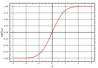
• Error function
  $${\displaystyle f(x)=\operatorname {erf} (x)={\frac {2}{\sqrt {\pi }}}\int _{0}^{x}e^{-t^{2}}\,dt}$$

  
• Generalised logistic function
  $${\displaystyle f(x)=\left(1+e^{-x}\right)^{-\alpha },\quad \alpha >0}$$

  
• Smoothstep function
  $${\displaystyle f(x)={\begin{cases}{\displaystyle \left(\int _{0}^{1}\left(1-u^{2}\right)^{N}du\right)^{-1}\int _{0}^{x}\left(1-u^{2}\right)^{N}\ du},&|x|\leq 1\\\\\operatorname {sgn}(x)&|x|\geq 1\\\end{cases}}\quad N\in \mathbb {Z} \geq 1}$$

  
• Some algebraic functions, for example
  $${\displaystyle f(x)={\frac {x}{\sqrt {1+x^{2}}}}}$$

  
• and in a more general form^[3]
  $${\displaystyle f(x)={\frac {x}{\left(1+|x|^{k}\right)^{1/k}}}}$$

  
• Up to shifts and scaling, many sigmoids are special cases of
  $${\displaystyle f(x)=\varphi (\varphi (x,\beta ),\alpha ),}$$

  
  where
  $${\displaystyle \varphi (x,\lambda )={\begin{cases}(1-\lambda x)^{1/\lambda }&\lambda \neq 0\\e^{-x}&\lambda =0\\\end{cases}}}$$

  
  is the inverse of the negative
  Box–Cox transformation
  , and ${\displaystyle \alpha <1}$ and ${\displaystyle \beta <1}$ are shape parameters.^[4]
• Smooth Interpolation^[5] normalized to (-1,1) and ${\displaystyle n}$ is the slope at zero:

using the hyperbolic tangent mentioned above.

Applications

Many natural processes, such as those of complex system learning curves, exhibit a progression from small beginnings that accelerates and approaches a climax over time. When a specific mathematical model is lacking, a sigmoid function is often used.^[6]

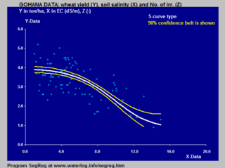
The van Genuchten–Gupta model is based on an inverted S-curve and applied to the response of crop yield to soil salinity.

Examples of the application of the logistic S-curve to the response of crop yield (wheat) to both the soil salinity and depth to water table in the soil are shown in modeling crop response in agriculture.

In

.

In

In

Hill–Langmuir equations

are sigmoid functions.

In computer graphics and real-time rendering, some of the sigmoid functions are used to blend colors or geometry between two values, smoothly and without visible seams or discontinuities.

pH scale

.

The logistic function can be calculated efficiently by utilizing

See also

References

Further reading

• Mitchell, Tom M. (1997). Machine Learning. WCB
  ISBN 978-0-07-042807-2
  .. (NB. In particular see "Chapter 4: Artificial Neural Networks" (in particular pp. 96–97) where Mitchell uses the word "logistic function" and the "sigmoid function" synonymously – this function he also calls the "squashing function" – and the sigmoid (aka logistic) function is used to compress the outputs of the "neurons" in multi-layer neural nets.)
• Humphrys, Mark. "Continuous output, the sigmoid function". Archived from the original on 2022-07-14. Retrieved 2022-07-14. (NB. Properties of the sigmoid, including how it can shift along axes and how its domain may be transformed.)

External links

• "Fitting of logistic S-curves (sigmoids) to data using SegRegA". Archived from the original on 2022-07-14.