Junction tree algorithm

The junction tree algorithm (also known as 'Clique Tree') is a method used in
Junction tree algorithm
Hugin algorithm
- If the graph is directed then moralize it to make it un-directed.
- Introduce the evidence.
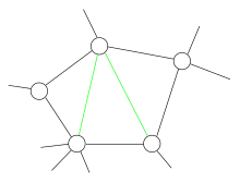
- Triangulate the graph to make it chordal.
- Construct a junction tree from the triangulated graph (we will call the vertices of the junction tree "supernodes").
- Propagate the probabilities along the junction tree (via belief propagation)
Note that this last step is inefficient for graphs of large treewidth. Computing the messages to pass between supernodes involves doing exact marginalization over the variables in both supernodes. Performing this algorithm for a graph with treewidth k will thus have at least one computation which takes time exponential in k. It is a message passing algorithm.[3] The Hugin algorithm takes fewer computations to find a solution compared to Shafer-Shenoy.
Shafer-Shenoy algorithm
- Computed recursively[3]
- Multiple recursions of the Shafer-Shenoy algorithm results in Hugin algorithm[4]
- Found by the message passing equation[4]
- Separator potentials are not stored[5]
The Shafer-Shenoy
Underlying theory

The first step concerns only
The second step is setting variables to their observed value. This is usually needed when we want to calculate conditional probabilities, so we fix the value of the random variables we condition on. Those variables are also said to be clamped to their particular value.

The third step is to ensure that graphs are made chordal if they aren't already chordal. This is the first essential step of the algorithm. It makes use of the following theorem:[8]
Theorem: For an undirected graph, G, the following properties are equivalent:
- Graph G is triangulated.
- The clique graph of G has a junction tree.
- There is an elimination ordering for G that does not lead to any added edges.
Thus, by triangulating a graph, we make sure that the corresponding junction tree exists. A usual way to do this, is to decide an elimination order for its nodes, and then run the Variable elimination algorithm. The variable elimination algorithm states that the algorithm must be run each time there is a different query.[1] This will result to adding more edges to the initial graph, in such a way that the output will be a chordal graph.
All chordal graphs have a junction tree.
Theorem: Given a triangulated graph, weight the edges of the clique graph by their cardinality, |A∩B|, of the intersection of the adjacent cliques A and B. Then any maximum-weight spanning tree of the clique graph is a junction tree.
So, to construct a junction tree we just have to extract a maximum weight spanning tree out of the clique graph. This can be efficiently done by, for example, modifying Kruskal's algorithm. The last step is to apply belief propagation to the obtained junction tree.[10]
Usage: A junction tree graph is used to visualize the probabilities of the problem. The tree can become a binary tree to form the actual building of the tree.[11] A specific use could be found in auto encoders, which combine the graph and a passing network on a large scale automatically.[12]
Inference Algorithms

Loopy belief propagation: A different method of interpreting complex graphs. The
Cutset conditioning: Used with smaller sets of variables.
References
- ^ a b c Paskin, Mark. "A Short Course on Graphical Models" (PDF). Stanford.
- ^ "The Inference Algorithm". www.dfki.de. Retrieved 2018-10-25.
- ^ a b c d "Recap on Graphical Models" (PDF).
- ^ a b c "Algorithms" (PDF). Massachusetts Institute of Technology. 2014.
- ^ Roweis, Sam (2004). "Hugin Inference Algorithm" (PDF). NYU.
- ^ "Algorithms for Inference" (PDF). Massachusetts Institute of Technology. 2014.
- ^ arXiv:1806.02373 [cs.AI].
- ^ a b Wainwright, Martin (31 March 2008). "Graphical models, message-passing algorithms, and variational methods: Part I" (PDF). Berkeley EECS. Retrieved 16 November 2016.
- ^ "Clique Graph". Retrieved 16 November 2016.
- ^ Barber, David (28 January 2014). "Probabilistic Modelling and Reasoning, The Junction Tree Algorithm" (PDF). University of Helsinki. Retrieved 16 November 2016.
- .
- Bibcode:2018arXiv180204364J.
- )
Further reading
- Lauritzen, Steffen L.; MR 0964177.
- S2CID 61247712.
- Huang, Cecil; Darwiche, Adnan (1996). "Inference in Belief Networks: A Procedural Guide". International Journal of Approximate Reasoning. 15 (3): 225–263. .
- Lepar, V., Shenoy, P. (1998). "A Comparison of Lauritzen-Spiegelhalter, Hugin, and Shenoy-Shafer Architectures for Computing Marginals of Probability Distributions." https://arxiv.org/ftp/arxiv/papers/1301/1301.7394.pdf
