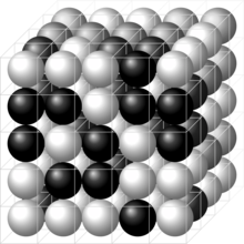
Lattice model (physics)

This article needs additional citations for verification. Please help improve this article by adding citations to reliable sources. Unsourced material may be challenged and removed. Find sources: "Lattice model" physics – news · newspapers · books · scholar · JSTOR (February 2016) (Learn how and when to remove this message)

In

are areas of study. Lattice models are also used to simulate the structure and dynamics of polymers.

Mathematical description

A number of lattice models can be described by the following data:

• A lattice ${\displaystyle \Lambda }$, often taken to be a lattice in ${\displaystyle d}$-dimensional Euclidean space ${\displaystyle \mathbb {R} ^{d}}$ or the ${\displaystyle d}$-dimensional torus if the lattice is periodic. Concretely, ${\displaystyle \Lambda }$ is often the cubic lattice. If two points on the lattice are considered 'nearest neighbours', then they can be connected by an edge, turning the lattice into a lattice graph. The vertices of ${\displaystyle \Lambda }$ are sometimes referred to as sites.
• A spin-variable space ${\displaystyle S}$. The configuration space ${\displaystyle {\mathcal {C}}}$ of possible system states is then the space of functions ${\displaystyle \sigma :\Lambda \rightarrow S}$. For some models, we might instead consider instead the space of functions ${\displaystyle \sigma :E\rightarrow S}$ where ${\displaystyle E}$ is the edge set of the graph defined above.
• An energy functional ${\displaystyle E:{\mathcal {C}}\rightarrow \mathbb {R} }$, which might depend on a set of additional parameters or 'coupling constants' ${\displaystyle \{g_{i}\}}$.

Examples

The Ising model is given by the usual cubic lattice graph ${\displaystyle G=(\Lambda ,E)}$ where ${\displaystyle \Lambda }$ is an infinite cubic lattice in ${\displaystyle \mathbb {R} ^{d}}$ or a period ${\displaystyle n}$ cubic lattice in ${\displaystyle T^{d}}$, and ${\displaystyle E}$ is the edge set of nearest neighbours (the same letter is used for the energy functional but the different usages are distinguishable based on context). The spin-variable space is ${\displaystyle S=\{+1,-1\}=\mathbb {Z} _{2}}$. The energy functional is

${\displaystyle E(\sigma )=-H\sum _{v\in \Lambda }\sigma (v)-J\sum _{\{v_{1},v_{2}\}\in E}\sigma (v_{1})\sigma (v_{2}).}$

The spin-variable space can often be described as a coset. For example, for the Potts model we have ${\displaystyle S=\mathbb {Z} _{n}}$. In the limit ${\displaystyle n\rightarrow \infty }$, we obtain the XY model which has ${\displaystyle S=SO(2)}$. Generalising the XY model to higher dimensions gives the ${\displaystyle n}$-vector model which has ${\displaystyle S=S^{n}=SO(n+1)/SO(n)}$.

Solvable models

We specialise to a lattice with a finite number of points, and a finite spin-variable space. This can be achieved by making the lattice periodic, with period ${\displaystyle n}$ in ${\displaystyle d}$ dimensions. Then the configuration space ${\displaystyle {\mathcal {C}}}$ is also finite. We can define the partition function

${\displaystyle Z=\sum _{\sigma \in {\mathcal {C}}}\exp(-\beta E(\sigma ))}$

and there are no issues of convergence (like those which emerge in field theory) since the sum is finite. In theory, this sum can be computed to obtain an expression which is dependent only on the parameters ${\displaystyle \{g_{i}\}}$ and ${\displaystyle \beta }$. In practice, this is often difficult due to non-linear interactions between sites. Models with a closed-form expression for the partition function are known as

.

Examples of exactly solvable models are the periodic 1D Ising model, and the periodic 2D Ising model with vanishing external magnetic field, ${\displaystyle H=0,}$ but for dimension ${\displaystyle d>2}$, the Ising model remains unsolved.

Mean field theory

Due to the difficulty of deriving exact solutions, in order to obtain analytic results we often must resort to

. This mean field may be spatially varying, or global.

Global mean field

The configuration space ${\displaystyle {\mathcal {C}}}$ of functions ${\displaystyle \sigma }$ is replaced by the convex hull of the spin space ${\displaystyle S}$, when ${\displaystyle S}$ has a realisation in terms of a subset of ${\displaystyle \mathbb {R} ^{m}}$. We'll denote this by ${\displaystyle \langle {\mathcal {C}}\rangle }$. This arises as in going to the mean value of the field, we have ${\displaystyle \sigma \mapsto \langle \sigma \rangle :={\frac {1}{|\Lambda |}}\sum _{v\in \Lambda }\sigma (v)}$.

As the number of lattice sites ${\displaystyle N=|\Lambda |\rightarrow \infty }$, the possible values of ${\displaystyle \langle \sigma \rangle }$ fill out the convex hull of ${\displaystyle S}$. By making a suitable approximation, the energy functional becomes a function of the mean field, that is, ${\displaystyle E(\sigma )\mapsto E(\langle \sigma \rangle ).}$ The partition function then becomes

${\displaystyle Z=\int _{\langle {\mathcal {C}}\rangle }d\langle \sigma \rangle e^{-\beta E(\langle \sigma \rangle )}\Omega (\langle \sigma \rangle )=:\int _{\langle {\mathcal {C}}\rangle }d\langle \sigma \rangle e^{-N\beta f(\langle \sigma \rangle )}.}$

As ${\displaystyle N\rightarrow \infty }$, that is, in the

tells us the integral is asymptotically dominated by the value at which ${\displaystyle f(\langle \sigma \rangle )}$ is minimised:

${\displaystyle Z\sim e^{-N\beta f(\langle \sigma \rangle _{0})}}$

where ${\displaystyle \langle \sigma \rangle _{0}}$ is the argument minimising ${\displaystyle f}$.

A simpler, but less mathematically rigorous approach which nevertheless sometimes gives correct results comes from linearising the theory about the mean field ${\displaystyle \langle \sigma \rangle }$. Writing configurations as ${\displaystyle \sigma (v)=\langle \sigma \rangle +\Delta \sigma (v)}$, truncating terms of ${\displaystyle {\mathcal {O}}(\Delta \sigma ^{2})}$ then summing over configurations allows computation of the partition function.

Such an approach to the periodic Ising model in ${\displaystyle d}$ dimensions provides insight into

.

Spatially varying mean field

Suppose the continuum limit of the lattice ${\displaystyle \Lambda }$ is ${\displaystyle \mathbb {R} ^{d}}$. Instead of averaging over all of ${\displaystyle \Lambda }$, we average over neighbourhoods of ${\displaystyle \mathbf {x} \in \mathbb {R} ^{d}}$. This gives a spatially varying mean field ${\displaystyle \langle \sigma \rangle :\mathbb {R} ^{d}\rightarrow \langle {\mathcal {C}}\rangle }$. We relabel ${\displaystyle \langle \sigma \rangle }$ with ${\displaystyle \phi }$ to bring the notation closer to field theory. This allows the partition function to be written as a path integral

${\displaystyle Z=\int {\mathcal {D}}\phi e^{-\beta F[\phi ]}}$

where the free energy ${\displaystyle F[\phi ]}$ is a

.

Examples

Condensed matter physics

• Ising model
• ANNNI model
• Potts model
• Chiral Potts model
• XY model
• Classical Heisenberg model
• n-vector model
• Vertex model
• Toda lattice
• cellular automata

Polymer physics

• Bond fluctuation model
• 2nd model

High energy physics

• QCD lattice model

See also

• Crystal structure
• Scaling limit
• QCD matter
• Lattice gas

References

• MR 0690578