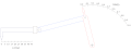
Linkage (mechanical)

A mechanical linkage is an assembly of systems connected to manage

.

Linkages may be constructed from open chains, closed chains, or a combination of open and closed chains. Each link in a chain is connected by a joint to one or more other links. Thus, a kinematic chain can be modeled as a graph in which the links are paths and the joints are vertices, which is called a linkage graph.

scissor lift

The movement of an ideal joint is generally associated with a subgroup of the group of

(DOF) of the joint. Mechanical linkages are usually designed to transform a given input force and movement into a desired output force and movement. The ratio of the output force to the input force is known as the . The speed ratio and mechanical advantage are defined so they yield the same number in an ideal linkage.

A kinematic chain, in which one link is fixed or stationary, is called a mechanism,^[2] and a linkage designed to be stationary is called a structure.

History

Archimedes^[3] applied geometry to the study of the lever. Into the 1500s the work of Archimedes and Hero of Alexandria were the primary sources of machine theory. It was Leonardo da Vinci who brought an inventive energy to machines and mechanism.^[4]

In the mid-1700s the

The work of Sylvester inspired A. B. Kempe, who showed that linkages for addition and multiplication could be assembled into a system that traced a given algebraic curve.^[6] Kempe's design procedure has inspired research at the intersection of geometry and computer science.^[7][8]

In the late 1800s F. Reuleaux, A. B. W. Kennedy, and L. Burmester formalized the analysis and synthesis of linkage systems using descriptive geometry, and P. L. Chebyshev introduced analytical techniques for the study and invention of linkages.^[5]

In the mid-1900s F. Freudenstein and G. N. Sandor^[9] used the newly developed digital computer to solve the loop equations of a linkage and determine its dimensions for a desired function, initiating the computer-aided design of linkages. Within two decades these computer techniques were integral to the analysis of complex machine systems^[10][11] and the control of robot manipulators.^[12]

R. E. Kaufman^[13][14] combined the computer's ability to rapidly compute the roots of polynomial equations with a graphical user interface to unite Freudenstein's techniques with the geometrical methods of Reuleaux and Burmester and form KINSYN, an interactive computer graphics system for linkage design

The modern study of linkages includes the analysis and design of articulated systems that appear in robots, machine tools, and cable driven and tensegrity systems. These techniques are also being applied to biological systems and even the study of proteins.

Mobility

The configuration of a system of rigid links connected by ideal joints is defined by a set of configuration parameters, such as the angles around a revolute joint and the slides along prismatic joints measured between adjacent links. The geometric constraints of the linkage allow calculation of all of the configuration parameters in terms of a minimum set, which are the input parameters. The number of input parameters is called the mobility, or

, of the linkage system.

A system of n rigid bodies moving in space has 6n degrees of freedom measured relative to a fixed frame. Include this frame in the count of bodies, so that mobility is independent of the choice of the fixed frame, then we have M = 6(N − 1), where N = n + 1 is the number of moving bodies plus the fixed body.

Joints that connect bodies in this system remove degrees of freedom and reduce mobility. Specifically, hinges and sliders each impose five constraints and therefore remove five degrees of freedom. It is convenient to define the number of constraints c that a joint imposes in terms of the joint's freedom f, where c = 6 − f. In the case of a hinge or slider, which are one degree of freedom joints, we have f = 1 and therefore c = 6 − 1 = 5.

Thus, the mobility of a linkage system formed from n moving links and j joints each with f_i, i = 1, ..., j, degrees of freedom can be computed as,

${\displaystyle M=6n-\sum _{i=1}^{j}(6-f_{i})=6(N-1-j)+\sum _{i=1}^{j}\ f_{i},}$

where N includes the fixed link. This is known as Kutzbach–Grübler's equation

There are two important special cases: (i) a simple open chain, and (ii) a simple closed chain. A simple open chain consists of n moving links connected end to end by j joints, with one end connected to a ground link. Thus, in this case N = j + 1 and the mobility of the chain is

${\displaystyle M=\sum _{i=1}^{j}\ f_{i}.}$

For a simple closed chain, n moving links are connected end-to-end by n+1 joints such that the two ends are connected to the ground link forming a loop. In this case, we have N=j and the mobility of the chain is

${\displaystyle M=\sum _{i=1}^{j}\ f_{i}-6.}$

An example of a simple open chain is a serial robot manipulator. These robotic systems are constructed from a series of links connected by six one degree-of-freedom revolute or prismatic joints, so the system has six degrees of freedom.

An example of a simple closed chain is the RSSR (revolute-spherical-spherical-revolute) spatial four-bar linkage. The sum of the freedom of these joints is eight, so the mobility of the linkage is two, where one of the degrees of freedom is the rotation of the coupler around the line joining the two S joints.

Planar and spherical movement

pliers exemplify a four-bar, one degree of freedom mechanical linkage. The adjustable base pivot makes this a two degree-of-freedom five-bar linkage

.

It is common practice to design the linkage system so that the movement of all of the bodies are constrained to lie on parallel planes, to form what is known as a planar linkage. It is also possible to construct the linkage system so that all of the bodies move on concentric spheres, forming a spherical linkage. In both cases, the degrees of freedom of the link is now three rather than six, and the constraints imposed by joints are now c = 3 − f.

In this case, the mobility formula is given by

${\displaystyle M=3(N-1-j)+\sum _{i=1}^{j}\ f_{i},}$

and we have the special cases,

• planar or spherical simple open chain,

${\displaystyle M=\sum _{i=1}^{j}\ f_{i},}$

• planar or spherical simple closed chain,

${\displaystyle M=\sum _{i=1}^{j}\ f_{i}-3.}$

An example of a planar simple closed chain is the planar four-bar linkage, which is a four-bar loop with four one degree-of-freedom joints and therefore has mobility M = 1.

Joints

The most familiar joints for linkage systems are the revolute, or hinged, joint denoted by an R, and the prismatic, or sliding, joint denoted by a P. Most other joints used for spatial linkages are modeled as combinations of revolute and prismatic joints. For example,

• the cylindric joint consists of an RP or PR serial chain constructed so that the axes of the revolute and prismatic joints are parallel,
• the universal joint consists of an RR serial chain constructed such that the axes of the revolute joints intersect at a 90° angle;
• the
  spherical joint
  consists of an RRR serial chain for which each of the hinged joint axes intersect in the same point;
• the planar joint can be constructed either as a planar RRR, RPR, and PPR serial chain that has three degrees-of-freedom.

Analysis and synthesis of linkages

The primary mathematical tool for the analysis of a linkage is known as the kinematic equations of the system. This is a sequence of rigid body transformation along a serial chain within the linkage that locates a floating link relative to the ground frame. Each serial chain within the linkage that connects this floating link to ground provides a set of equations that must be satisfied by the configuration parameters of the system. The result is a set of non-linear equations that define the configuration parameters of the system for a set of values for the input parameters.

.

Planar one degree-of-freedom linkages

The mobility formula provides a way to determine the number of links and joints in a planar linkage that yields a one degree-of-freedom linkage. If we require the mobility of a planar linkage to be M = 1 and f_i = 1, the result is

${\displaystyle M=3(N-1-j)+j=1,\!}$

or

${\displaystyle j={\frac {3}{2}}N-2.\!}$

This formula shows that the linkage must have an even number of links, so we have

• N = 2, j = 1: this is a two-bar linkage known as the lever;
• N = 4, j = 4: this is the four-bar linkage;
• N = 6, j = 7: this is a six-bar linkage [ it has two links that have three joints, called ternary links, and there are two topologies of this linkage depending how these links are connected. In the Watt topology, the two ternary links are connected by a joint. In the Stephenson topology the two ternary links are connected by binary links;^[15]
• N = 8, j = 10: the eight-bar linkage has 16 different topologies;
• N = 10, j = 13: the 10-bar linkage has 230 different topologies,
• N = 12, j = 16: the 12-bar has 6856 topologies.

See Sunkari and Schmidt^[16] for the number of 14- and 16-bar topologies, as well as the number of linkages that have two, three and four degrees-of-freedom.

The planar four-bar linkage is probably the simplest and most common linkage. It is a one degree-of-freedom system that transforms an input crank rotation or slider displacement into an output rotation or slide.

Examples of four-bar linkages are:

• the crank-rocker, in which the input crank fully rotates and the output link rocks back and forth;
• the slider-crank, in which the input crank rotates and the output slide moves back and forth;
• drag-link mechanisms, in which the input crank fully rotates and drags the output crank in a fully rotational movement.

Other interesting linkages

• Pantograph (four-bar, two DOF)
• Five bar linkages often have meshing gears for two of the links, creating a one DOF linkage. They can provide greater power transmission with more design flexibility than four-bar linkages.
• Jansen's linkage is an eight-bar leg mechanism that was invented by kinetic sculptor Theo Jansen.
• Klann linkage is a six-bar linkage that forms a leg mechanism;
• Toggle mechanisms are four-bar linkages that are dimensioned so that they can fold and lock. The toggle positions are determined by the colinearity of two of the moving links.^[17] The linkage is dimensioned so that the linkage reaches a toggle position just before it folds. The high mechanical advantage allows the input crank to deform the linkage just enough to push it beyond the toggle position. This locks the input in place. Toggle mechanisms are used as clamps.

Straight line mechanisms

• James Watt's
  parallel motion and Watt's linkage
• Peaucellier–Lipkin linkage, the first planar linkage to create a perfect straight line output from rotary input; eight-bar, one DOF.
• A Scott Russell linkage, which converts linear motion, to (almost) linear motion in a line perpendicular to the input.
• Chebyshev linkage, which provides nearly straight motion of a point with a four-bar linkage.
• Hoekens linkage
  , which provides nearly straight motion of a point with a four-bar linkage.
• Sarrus linkage, which provides motion of one surface in a direction normal to another.
• Hart's inversor, which provides a perfect straight line motion without sliding guides.^[18]

Biological linkages

Linkage systems are widely distributed in animals. The most thorough overview of the different types of linkages in animals has been provided by Mees Muller,[19] who also designed a new classification system which is especially well suited for biological systems. A well-known example is the cruciate ligaments of the knee.

An important difference between biological and engineering linkages is that revolving bars are rare in biology and that usually only a small range of the theoretically possible is possible due to additional functional constraints (especially the necessity to deliver blood).^[20] Biological linkages frequently are compliant. Often one or more bars are formed by ligaments, and often the linkages are three-dimensional. Coupled linkage systems are known, as well as five-, six-, and even seven-bar linkages.^[19] Four-bar linkages are by far the most common though.

Linkages can be found in joints, such as the knee of tetrapods, the hock of sheep, and the cranial mechanism of birds and reptiles. The latter is responsible for the upward motion of the upper bill in many birds.

Linkage mechanisms are especially frequent and manifold in the head of

.

Linkages are also present as locking mechanisms, such as in the knee of the horse, which enables the animal to sleep standing, without active muscle contraction. In

pivot feeding

, used by certain bony fishes, a four-bar linkage at first locks the head in a ventrally bent position by the alignment of two bars. The release of the locking mechanism jets the head up and moves the mouth toward the prey within 5–10 ms.

Image gallery

[21] ^{[22] [23]}

• 
  Rocker-slider function generator approximating the function Log(u) for 1 < u < 10.
• 
  Slider-rocker function generator approximating the function Tan(u) for 0 < u < 45°.
• 
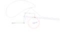
  Fixed and moving centrodes of a four-bar linkage
• 
  Rack-and-pinion four-bar linkage
• 
  RTRTR mechanism
• 
  RTRTR mechanism
• 
  Gear five-bar mechanisms
• 
  3D slider-crank mechanism
• 
  Animated Pinocchio character
• 
• 
  Crawford conicograph
• 
  Outward folding deployable mechanism
• 
  Inward folding deployable mechanism

See also

References

Further reading

• Bryant, John; Sangwin, Chris (2008).
  ISBN 978-0-691-13118-4
  . — Connections between mathematical and real-world mechanical models, historical development of precision machining, some practical advice on fabricating physical models, with ample illustrations and photographs
• Erdman, Arthur G.; Sandor, George N. (1984). Mechanism Design: Analysis and Synthesis. Prentice-Hall.
  ISBN 0-13-572396-5
  .
• Hartenberg, R.S. & J. Denavit (1964) Kinematic synthesis of linkages, New York: McGraw-Hill — Online link from Cornell University.
• ISBN 978-0-8018-8814-4
  . — "Linkages: a peculiar fascination" (Chapter 14) is a discussion of mechanical linkage usage in American mathematical education, includes extensive references
• How to Draw a Straight Line — Historical discussion of linkage design from Cornell University
• Parmley, Robert. (2000). "Section 23: Linkage." Illustrated Sourcebook of Mechanical Components. New York: McGraw Hill.
  ISBN 0-07-048617-4
  Drawings and discussion of various linkages.
• Sclater, Neil. (2011). "Linkages: Drives and Mechanisms." Mechanisms and Mechanical Devices Sourcebook. 5th ed. New York: McGraw Hill. pp. 89–129.
  ISBN 978-0-07-170442-7
  . Drawings and designs of various linkages.

External links

Wikimedia Commons has media related to Linkage (mechanical).

• Kinematic Models for Design Digital Library (KMODDL) — Major web resource for kinematics. Movies and photos of hundreds of working mechanical-systems models in the Reuleaux Collection of Mechanisms and Machines at Cornell University, plus 5 other major collections. Includes an e-book library of dozens of classic texts on mechanical design and engineering. Includes CAD models and stereolithographic files for selected mechanisms.
• Digital Mechanism and Gear Library (DMG-Lib) (in German: Digitale Mechanismen- und Getriebebibliothek) — Online library about linkages and cams (mostly in German)
• Linkage calculations
• Introductory linkage lecture
• Virtual Mechanisms Animated by Java
• Linkage-based Drawing Apparatus by Robert Howsare
• (ASOM) Analysis, synthesis and optimization of multibar linkages
• Linkage animations on mechanicaldesign101.com include planar and spherical four-bar and six-bar linkages.
• Animations of planar and spherical four-bar linkages.
• Animation of Bennett's linkage.
• Example of a six-bar function generator that computes the elevation angle for a given range.
• Animations of six-bar linkage for a bicycle suspension.
• A variety of six-bar linkage designs.
• Introduction to Linkages
• An open source planar linkage mechanism simulation and mechanical synthesis system.