The probabilities associated with all (hypothetical) values must be non-negative and sum up to 1,
and
Thinking of probability as mass helps to avoid mistakes since the physical mass is conserved as is the total probability for all hypothetical outcomes .
Measure theoretic formulation
A probability mass function of a discrete random variable can be seen as a special case of two more general measure theoretic constructions:
the distribution of and the probability density function of with respect to the counting measure. We make this more precise below.
Suppose that is a probability space
and that is a measurable space whose underlying
σ-algebra
is discrete, so in particular contains singleton sets of . In this setting, a random variable is discrete provided its image is countable.
The pushforward measure—called the distribution of in this context—is a probability measure on whose restriction to singleton sets induces the probability mass function (as mentioned in the previous section) since for each .
Now suppose that is a measure space equipped with the counting measure μ. The probability density function of with respect to the counting measure, if it exists, is the
Radon–Nikodym derivative
of the pushforward measure of (with respect to the counting measure), so and is a function from to the non-negative reals. As a consequence, for any we have
demonstrating that is in fact a probability mass function.
When there is a natural order among the potential outcomes , it may be convenient to assign numerical values to them (or n-tuples in case of a discrete multivariate random variable) and to consider also values not in the image of . That is, may be defined for all real numbers and for all as shown in the figure.
The image of has a
countable
subset on which the probability mass function is one. Consequently, the probability mass function is zero for all but a countable number of values of .
The discontinuity of probability mass functions is related to the fact that the cumulative distribution function of a discrete random variable is also discontinuous. If is a discrete random variable, then means that the casual event is certain (it is true in 100% of the occurrences); on the contrary, means that the casual event is always impossible. This statement isn't true for a
continuous random variable
, for which for any possible . Discretization is the process of converting a continuous random variable into a discrete one.
Bernoulli distribution: ber(p) , is used to model an experiment with only two possible outcomes. The two outcomes are often encoded as 1 and 0.
An example of the Bernoulli distribution is tossing a coin. Suppose that is the sample space of all outcomes of a single toss of a fair coin, and is the random variable defined on assigning 0 to the category "tails" and 1 to the category "heads". Since the coin is fair, the probability mass function is
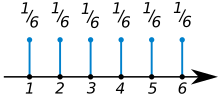
Binomial distribution, models the number of successes when someone draws n times with replacement. Each draw or experiment is independent, with two possible outcomes. The associated probability mass function is . The probability mass function of a fair die. All the numbers on the die have an equal chance of appearing on top when the die stops rolling.An example of the binomial distribution is the probability of getting exactly one 6 when someone rolls a fair die three times.
Geometric distribution describes the number of trials needed to get one success. Its probability mass function is .An example is tossing a coin until the first "heads" appears. denotes the probability of the outcome "heads", and denotes the number of necessary coin tosses. Other distributions that can be modeled using a probability mass function are the categorical distribution (also known as the generalized Bernoulli distribution) and the multinomial distribution.
If the discrete distribution has two or more categories one of which may occur, whether or not these categories have a natural ordering, when there is only a single trial (draw) this is a categorical distribution.
An example of a multivariate discrete distribution, and of its probability mass function, is provided by the multinomial distribution. Here the multiple random variables are the numbers of successes in each of the categories after a given number of trials, and each non-zero probability mass gives the probability of a certain combination of numbers of successes in the various categories.
Infinite
The following exponentially declining distribution is an example of a distribution with an infinite number of possible outcomes—all the positive integers:
Despite the infinite number of possible outcomes, the total probability mass is 1/2 + 1/4 + 1/8 + ⋯ = 1, satisfying the unit total probability requirement for a probability distribution.
Two or more discrete random variables have a joint probability mass function, which gives the probability of each possible combination of realizations for the random variables.


![{\displaystyle p:\mathbb {R} \to [0,1]}](https://wikimedia.org/api/rest_v1/media/math/render/svg/46d0bfcc5e761714acd5cd8f1cdad03533eb72fa)