t-distributed stochastic neighbor embedding

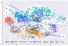
t-distributed stochastic neighbor embedding (t-SNE) is a

While t-SNE plots often seem to display clusters, the visual clusters can be influenced strongly by the chosen parameterization and therefore a good understanding of the parameters for t-SNE is necessary. Such "clusters" can be shown to even appear in non-clustered data,^[11] and thus may be false findings. Interactive exploration may thus be necessary to choose parameters and validate results.^[12][13] It has been demonstrated that t-SNE is often able to recover well-separated clusters, and with special parameter choices, approximates a simple form of spectral clustering.^[14]

For a data set with n elements, t-SNE runs in O(n²) time and requires O(n²) space.^[15]

Details

Given a set of ${\displaystyle N}$ high-dimensional objects ${\displaystyle \mathbf {x} _{1},\dots ,\mathbf {x} _{N}}$, t-SNE first computes probabilities ${\displaystyle p_{ij}}$ that are proportional to the similarity of objects ${\displaystyle \mathbf {x} _{i}}$ and ${\displaystyle \mathbf {x} _{j}}$, as follows.

For ${\displaystyle i\neq j}$, define

${\displaystyle p_{j\mid i}={\frac {\exp(-\lVert \mathbf {x} _{i}-\mathbf {x} _{j}\rVert ^{2}/2\sigma _{i}^{2})}{\sum _{k\neq i}\exp(-\lVert \mathbf {x} _{i}-\mathbf {x} _{k}\rVert ^{2}/2\sigma _{i}^{2})}}}$

and set ${\displaystyle p_{i\mid i}=0}$. Note the above denominator ensures ${\displaystyle \sum _{j}p_{j\mid i}=1}$ for all ${\displaystyle i}$.

As van der Maaten and Hinton explained: "The similarity of datapoint ${\displaystyle x_{j}}$ to datapoint ${\displaystyle x_{i}}$ is the conditional probability, ${\displaystyle p_{j|i}}$, that ${\displaystyle x_{i}}$ would pick ${\displaystyle x_{j}}$ as its neighbor if neighbors were picked in proportion to their probability density under a Gaussian centered at ${\displaystyle x_{i}}$."^[2]

Now define

${\displaystyle p_{ij}={\frac {p_{j\mid i}+p_{i\mid j}}{2N}}}$

This is motivated because ${\displaystyle p_{i}}$ and ${\displaystyle p_{j}}$ from the N samples are estimated as 1/N, so the conditional probability can be written as ${\displaystyle p_{i\mid j}=Np_{ij}}$ and ${\displaystyle p_{j\mid i}=Np_{ji}}$ . Since ${\displaystyle p_{ij}=p_{ji}}$, you can obtain previous formula.

Also note that ${\displaystyle p_{ii}=0}$ and ${\displaystyle \sum _{i,j}p_{ij}=1}$.

The bandwidth of the

${\displaystyle \sigma _{i}}$

${\displaystyle \sigma _{i}}$

Since the Gaussian kernel uses the Euclidean distance ${\displaystyle \lVert x_{i}-x_{j}\rVert }$, it is affected by the curse of dimensionality, and in high dimensional data when distances lose the ability to discriminate, the ${\displaystyle p_{ij}}$ become too similar (asymptotically, they would converge to a constant). It has been proposed to adjust the distances with a power transform, based on the intrinsic dimension of each point, to alleviate this.^[16]

t-SNE aims to learn a ${\displaystyle d}$-dimensional map ${\displaystyle \mathbf {y} _{1},\dots ,\mathbf {y} _{N}}$ (with ${\displaystyle \mathbf {y} _{i}\in \mathbb {R} ^{d}}$ and ${\displaystyle d}$ typically chosen as 2 or 3) that reflects the similarities ${\displaystyle p_{ij}}$ as well as possible. To this end, it measures similarities ${\displaystyle q_{ij}}$ between two points in the map ${\displaystyle \mathbf {y} _{i}}$ and ${\displaystyle \mathbf {y} _{j}}$, using a very similar approach. Specifically, for ${\displaystyle i\neq j}$, define ${\displaystyle q_{ij}}$ as

${\displaystyle q_{ij}={\frac {(1+\lVert \mathbf {y} _{i}-\mathbf {y} _{j}\rVert ^{2})^{-1}}{\sum _{k}\sum _{l\neq k}(1+\lVert \mathbf {y} _{k}-\mathbf {y} _{l}\rVert ^{2})^{-1}}}}$

and set ${\displaystyle q_{ii}=0}$. Herein a heavy-tailed

The locations of the points ${\displaystyle \mathbf {y} _{i}}$ in the map are determined by minimizing the (non-symmetric) Kullback–Leibler divergence of the distribution ${\displaystyle P}$ from the distribution ${\displaystyle Q}$, that is:

${\displaystyle \mathrm {KL} \left(P\parallel Q\right)=\sum _{i\neq j}p_{ij}\log {\frac {p_{ij}}{q_{ij}}}}$

The minimization of the Kullback–Leibler divergence with respect to the points ${\displaystyle \mathbf {y} _{i}}$ is performed using gradient descent. The result of this optimization is a map that reflects the similarities between the high-dimensional inputs.

Software

• The R package Rtsne implements t-SNE in R.
• ELKI contains tSNE, also with Barnes-Hut approximation
• scikit-learn, a popular machine learning library in Python implements t-SNE with both exact solutions and the Barnes-Hut approximation.
• Tensorboard, the visualization kit associated with TensorFlow, also implements t-SNE (online version)

References

- Neural Information Processing Systems.
- ^ a b van der Maaten, L.J.P.; Hinton, G.E. (Nov 2008). "Visualizing Data Using t-SNE" (PDF). Journal of Machine Learning Research. 9: 2579–2605.
- ^ Gashi, I.; Stankovic, V.; Leita, C.; Thonnard, O. (2009). "An Experimental Study of Diversity with Off-the-shelf AntiVirus Engines". Proceedings of the IEEE International Symposium on Network Computing and Applications: 4–11.
- ^ Hamel, P.; Eck, D. (2010). "Learning Features from Music Audio with Deep Belief Networks". Proceedings of the International Society for Music Information Retrieval Conference: 339–344.
- PMID 20175497.
- PMID 19153135.
- S2CID 67926902.
- ISBN 978-3-319-46681-1.
- S2CID 208329378.
- S2CID 8074617.
- ^ "K-means clustering on the output of t-SNE". Cross Validated. Retrieved 2018-04-16.
- S2CID 353336.
- . Retrieved 4 December 2017.
- arXiv:1706.02582 [cs.LG].
- ^ Pezzotti, Nicola. "Approximated and User Steerable tSNE for Progressive Visual Analytics" (PDF). Retrieved 31 August 2023.
- .
External links
- Visualizing Data Using t-SNE, Google Tech Talk about t-SNE
- Implementations of t-SNE in various languages, A link collection maintained by Laurens van der Maaten