Mixed model
| Part of a series on |
| Regression analysis |
|---|
| Models |
| Estimation |
|
| Background |
|
A mixed model, mixed-effects model or mixed error-component model is a
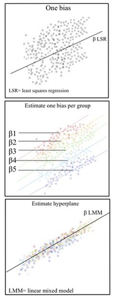
These models are useful in a wide variety of disciplines in the physical, biological and social sciences. They are particularly useful in settings where repeated measurements are made on the same statistical units (longitudinal study), or where measurements are made on clusters of related statistical units.[2] Mixed models are often preferred over traditional analysis of variance regression models because of their flexibility in dealing with missing values and uneven spacing of repeated measurements.[3] The Mixed model analysis allows measurements to be explicitly modeled in a wider variety of correlation and variance-covariance structures.This page will discuss mainly linear mixed-effects models rather than generalized linear mixed models or nonlinear mixed-effects models.[4]
Qualitative Description
Linear mixed models (LMMs) are
Non-independent sets are ones in which the variability between outcomes is due to correlations within groups or between groups. Mixed models properly account for nest structures/hierarchical data structures where observations are influenced by their nested associations. For example, when studying education methods involving multiple schools, there are multiple levels of variables to consider. The individual level/lower level comprises individual students or teachers within the school. The observations obtained from this student/teacher is nested within their school. For example, Student A is a unit within the School A. The next higher level is the school. At the higher level, the school contains multiple individual students and teachers. The school level influences the observations obtained from the students and teachers. For Example, School A and School B are the higher levels each with its set of Student A and Student B respectively. This represents a hierarchical data scheme. A solution to modeling hierarchical data is using linear mixed models.

LMMs allow us to understand the important effects between and within levels while incorporating the corrections for standard errors for non-independence embedded in the data structure.[4][5]
The Fixed Effect
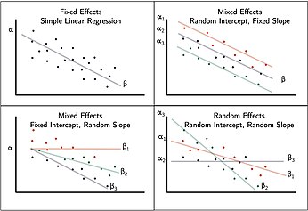
Fixed effects encapsulate the tendencies/trends that are consistent at the levels of primary interest. These effects are considered fixed because they are non-random and assumed to be constant for the population being studied.[5] For example, when studying education a fixed effect could represent overall school level effects that are consistent across all schools.
While the hierarchy of the data set is typically obvious, the specific fixed effects that affect the average responses for all subjects must be specified. Some fixed effect coefficients are sufficient without corresponding random effects where as other fixed coefficients only represent an average where the individual units are random. These may be determined by incorporating random
In most situations, several related models are considered and the model that best represents a universal model is adopted.
The Random Effect, ε
A key component of the mixed model is the incorporation of random effects with the fixed effect. Fixed effects are often fitted to represent the underlying model. In Linear mixed models, the true
History and current status

Ronald Fisher introduced random effects models to study the correlations of trait values between relatives.[9] In the 1950s, Charles Roy Henderson provided
Definition
In
where
- is a known vector of observations, with mean ;
- is an unknown vector of fixed effects;
- is an unknown vector of random effects, with mean and variance–covariance matrix ;
- is an unknown vector of random errors, with mean and variance ;
- is the known design matrix for the fixed effects relating the observations to , respectively
- is the known design matrix for the random effects relating the observations to , respectively.
Estimation
The joint density of and can be written as: . Assuming normality, , and , and maximizing the joint density over and , gives Henderson's "mixed model equations" (MME) for linear mixed models:[10][12][17]
The solutions to the MME, and are best linear unbiased estimates and predictors for and , respectively. This is a consequence of the Gauss–Markov theorem when the conditional variance of the outcome is not scalable to the identity matrix. When the conditional variance is known, then the inverse variance weighted least squares estimate is best linear unbiased estimates. However, the conditional variance is rarely, if ever, known. So it is desirable to jointly estimate the variance and weighted parameter estimates when solving MMEs.
One method used to fit such mixed models is that of the

There are several other methods to fit mixed models, including using an MEM initially, and then Newton-Raphson (used by R package nlme[21]'s lme()), penalized least squares to get a profiled log likelihood only depending on the (low-dimensional) variance-covariance parameters of , i.e., its cov matrix , and then modern direct optimization for that reduced objective function (used by R's lme4[22] package lmer() and the Julia package MixedModels.jl) and direct optimization of the likelihood (used by e.g. R's glmmTMB). Notably, while the canonical form proposed by Henderson is useful for theory, many popular software packages use a different formulation for numerical computation in order to take advantage of sparse matrix methods (e.g. lme4 and MixedModels.jl).
See also
- Nonlinear mixed-effects model
- Fixed effects model
- Generalized linear mixed model
- Linear regression
- Mixed-design analysis of variance
- Multilevel model
- Random effects model
- Repeated measures design
- Empirical Bayes method
References
- ISBN 978-0-470-51886-1.
- ^ PMID 35116198.
- PMID 24473328.
- ^ a b Seltman, Howard (2016). Experimental Design and Analysis. Vol. 1. pp. 357–378.
- ^ a b "Introduction to Linear Mixed Models". Advanced Research Computing Statistical Methods and Data Analytics. UCLA Statistical Consulting Group. 2021.
- ^ a b Kreft & de Leeuw, J. Introducing multilevel modeling. London:Sage.
- ^ a b Raudenbush, Bryk, S.W, A.S (2002). Hierarchical Linear Models: Applications and Data Analysis Methods. Thousand Oaks, CA: Sage.
{{cite book}}: CS1 maint: multiple names: authors list (link) - ^ a b Snijders, Bosker, T.A.B, R.J (2012). Multilevel analysis: An introduction to basic and advanced multilevel modeling. Vol. 2nd edition. London:Sage.
{{cite book}}: CS1 maint: multiple names: authors list (link) - S2CID 181213898.
- ^ JSTOR 2245695.
- JSTOR 2527669.
- ^ United States National Academy of Sciences.
- JSTOR 2685241.
- ^ Anderson, R.J (2016). ""MLB analytics guru who could be the next Nate Silver has a revolutionary new stat"".
- ^ Obenchain, Lilly, Bob, Eli (1993). "Data Analysis and Information Visualization" (PDF). MWSUG.
{{cite book}}: CS1 maint: multiple names: authors list (link) - PMID 27018471.
- . Retrieved 17 August 2014.
- .
- PMID 7168798.
- ^ Fitzmaurice, Garrett M.; Laird, Nan M.; Ware, James H. (2004). Applied Longitudinal Analysis. John Wiley & Sons. pp. 326–328.
- ISBN 0-387-98957-9.
- hdl:2027.42/146808.
Further reading
- Gałecki, Andrzej; Burzykowski, Tomasz (2013). Linear Mixed-Effects Models Using R: A Step-by-Step Approach. New York: Springer. ISBN 978-1-4614-3900-4.
- Milliken, G. A.; Johnson, D. E. (1992). Analysis of Messy Data: Vol. I. Designed Experiments. New York: Chapman & Hall.
- West, B. T.; Welch, K. B.; Galecki, A. T. (2007). Linear Mixed Models: A Practical Guide Using Statistical Software. New York: Chapman & Hall/CRC.


