
Least squares
| Part of a series on |
| Regression analysis |
|---|
| Models |
| Estimation |
|
| Background |
|


The method of least squares is a
The most important application is in
Least squares problems fall into two categories: linear or
When the observations come from an
The following discussion is mostly presented in terms of
The least-squares method was officially discovered and published by Adrien-Marie Legendre (1805),[2] though it is usually also co-credited to Carl Friedrich Gauss (1809),[3][4] who contributed significant theoretical advances to the method,[4] and may have also used it in his earlier work in 1794 and 1795.[5][4]
History
Founding
The method of least squares grew out of the fields of astronomy and geodesy, as scientists and mathematicians sought to provide solutions to the challenges of navigating the Earth's oceans during the Age of Discovery. The accurate description of the behavior of celestial bodies was the key to enabling ships to sail in open seas, where sailors could no longer rely on land sightings for navigation.
The method was the culmination of several advances that took place during the course of the eighteenth century:[6]
- The combination of different observations as being the best estimate of the true value; errors decrease with aggregation rather than increase, perhaps first expressed by Roger Cotes in 1722.
- The combination of different observations taken under the same conditions contrary to simply trying one's best to observe and record a single observation accurately. The approach was known as the method of averages. This approach was notably used by Tobias Mayer while studying the librations of the Moon in 1750, and by Pierre-Simon Laplace in his work in explaining the differences in motion of Jupiter and Saturn in 1788.
- The combination of different observations taken under different conditions. The method came to be known as the method of least absolute deviation. It was notably performed by Roger Joseph Boscovich in his work on the shape of the Earth in 1757 and by Pierre-Simon Laplacefor the same problem in 1789 and 1799.
- The development of a criterion that can be evaluated to determine when the solution with the minimum error has been achieved. Laplace tried to specify a mathematical form of the probability density for the errors and define a method of estimation that minimizes the error of estimation. For this purpose, Laplace used a symmetric two-sided exponential distribution we now call Laplace distribution to model the error distribution, and used the sum of absolute deviation as error of estimation. He felt these to be the simplest assumptions he could make, and he had hoped to obtain the arithmetic mean as the best estimate. Instead, his estimator was the posterior median.
The method

The first clear and concise exposition of the method of least squares was published by Legendre in 1805.[7] The technique is described as an algebraic procedure for fitting linear equations to data and Legendre demonstrates the new method by analyzing the same data as Laplace for the shape of the Earth. Within ten years after Legendre's publication, the method of least squares had been adopted as a standard tool in astronomy and geodesy in France, Italy, and Prussia, which constitutes an extraordinarily rapid acceptance of a scientific technique.[6]
In 1809
An early demonstration of the strength of Gauss's method came when it was used to predict the future location of the newly discovered asteroid Ceres. On 1 January 1801, the Italian astronomer Giuseppe Piazzi discovered Ceres and was able to track its path for 40 days before it was lost in the glare of the Sun. Based on these data, astronomers desired to determine the location of Ceres after it emerged from behind the Sun without solving Kepler's complicated nonlinear equations of planetary motion. The only predictions that successfully allowed Hungarian astronomer Franz Xaver von Zach to relocate Ceres were those performed by the 24-year-old Gauss using least-squares analysis.
In 1810, after reading Gauss's work, Laplace, after proving the central limit theorem, used it to give a large sample justification for the method of least squares and the normal distribution. In 1822, Gauss was able to state that the least-squares approach to regression analysis is optimal in the sense that in a linear model where the errors have a mean of zero, are uncorrelated, and have equal variances, the best linear unbiased estimator of the coefficients is the least-squares estimator. This result is known as the Gauss–Markov theorem.
The idea of least-squares analysis was also independently formulated by the American Robert Adrain in 1808. In the next two centuries workers in the theory of errors and in statistics found many different ways of implementing least squares.[9]
Problem statement
The objective consists of adjusting the parameters of a model function to best fit a data set. A simple data set consists of n points (data pairs) , i = 1, …, n, where is an


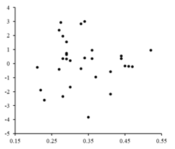
The residuals are plotted against corresponding values. The random fluctuations about indicate a linear model is appropriate.


The least-squares method finds the optimal parameter values by minimizing the


In the simplest case and the result of the least-squares method is the arithmetic mean of the input data.

An example of a model in two dimensions is that of the straight line. Denoting the y-intercept as and the slope as , the model function is given by . See linear least squares for a fully worked out example of this model.


A data point may consist of more than one independent variable. For example, when fitting a plane to a set of height measurements, the plane is a function of two independent variables, x and z, say. In the most general case there may be one or more independent variables and one or more dependent variables at each data point.
To the right is a residual plot illustrating random fluctuations about , indicating that a linear model is appropriate. is an independent, random variable.[10]


If the residual points had some sort of a shape and were not randomly fluctuating, a linear model would not be appropriate. For example, if the residual plot had a parabolic shape as seen to the right, a parabolic model would be appropriate for the data. The residuals for a parabolic model can be calculated via .[10]


Limitations
This regression formulation considers only observational errors in the dependent variable (but the alternative total least squares regression can account for errors in both variables). There are two rather different contexts with different implications:
- Regression for prediction. Here a model is fitted to provide a prediction rule for application in a similar situation to which the data used for fitting apply. Here the dependent variables corresponding to such future application would be subject to the same types of observation error as those in the data used for fitting. It is therefore logically consistent to use the least-squares prediction rule for such data.
- Regression for fitting a "true relationship". In standard hypothesis testing and confidence intervals that take into account the presence of observation errors in the independent variables.[11] An alternative approach is to fit a model by total least squares; this can be viewed as taking a pragmatic approach to balancing the effects of the different sources of error in formulating an objective function for use in model-fitting.
Solving the least squares problem
The


The gradient equations apply to all least squares problems. Each particular problem requires particular expressions for the model and its partial derivatives.[12]
Linear least squares
A regression model is a linear one when the model comprises a linear combination of the parameters, i.e.,


Letting and putting the independent and dependent variables in matrices and , respectively, we can compute the least squares in the following way. Note that is the set of all data.[12][13]


The gradient of the loss is:

Setting the gradient of the loss to zero and solving for , we get:[13][12]


Non-linear least squares
There is, in some cases, a


The Jacobian J is a function of constants, the independent variable and the parameters, so it changes from one iteration to the next. The residuals are given by

To minimize the sum of squares of , the gradient equation is set to zero and solved for :


The normal equations are written in matrix notation as

These are the defining equations of the Gauss–Newton algorithm.
Differences between linear and nonlinear least squares
- The model function, f, in LLSQ (linear least squares) is a linear combination of parameters of the form The model may represent a straight line, a parabola or any other linear combination of functions. In NLLSQ (nonlinear least squares) the parameters appear as functions, such as and so forth. If the derivatives are either constant or depend only on the values of the independent variable, the model is linear in the parameters. Otherwise the model is nonlinear.
- Need initial values for the parameters to find the solution to a NLLSQ problem; LLSQ does not require them.
- Solution algorithms for NLLSQ often require that the Jacobian can be calculated similar to LLSQ. Analytical expressions for the partial derivatives can be complicated. If analytical expressions are impossible to obtain either the partial derivatives must be calculated by numerical approximation or an estimate must be made of the Jacobian, often via finite differences.
- Non-convergence (failure of the algorithm to find a minimum) is a common phenomenon in NLLSQ.
- LLSQ is globally concave so non-convergence is not an issue.
- Solving NLLSQ is usually an iterative process which has to be terminated when a convergence criterion is satisfied. LLSQ solutions can be computed using direct methods, although problems with large numbers of parameters are typically solved with iterative methods, such as the Gauss–Seidelmethod.
- In LLSQ the solution is unique, but in NLLSQ there may be multiple minima in the sum of squares.
- Under the condition that the errors are uncorrelated with the predictor variables, LLSQ yields unbiased estimates, but even under that condition NLLSQ estimates are generally biased.


These differences must be considered whenever the solution to a nonlinear least squares problem is being sought.[12]
Example
Consider a simple example drawn from physics. A spring should obey Hooke's law which states that the extension of a spring y is proportional to the force, F, applied to it.

constitutes the model, where F is the independent variable. In order to estimate the


There are many methods we might use to estimate the unknown parameter k. Since the n equations in the m variables in our data comprise an overdetermined system with one unknown and n equations, we estimate k using least squares. The sum of squares to be minimized is

The least squares estimate of the force constant, k, is given by

We assume that applying force causes the spring to expand. After having derived the force constant by least squares fitting, we predict the extension from Hooke's law.
Uncertainty quantification
In a least squares calculation with unit weights, or in linear regression, the variance on the jth parameter, denoted , is usually estimated with

![{\displaystyle \operatorname {var} ({\hat {\beta }}_{j})=\sigma ^{2}\left(\left[X^{\mathsf {T}}X\right]^{-1}\right)_{jj}\approx {\hat {\sigma }}^{2}C_{jj},}](https://wikimedia.org/api/rest_v1/media/math/render/svg/d85cf89d392a9c191ff1fe3429654bd748a02b2b)


where the true error variance σ2 is replaced by an estimate, the reduced chi-squared statistic, based on the minimized value of the residual sum of squares (objective function), S. The denominator, n − m, is the statistical degrees of freedom; see effective degrees of freedom for generalizations.[12] C is the covariance matrix.
Statistical testing
If the
It is necessary to make assumptions about the nature of the experimental errors to test the results statistically. A common assumption is that the errors belong to a normal distribution. The central limit theorem supports the idea that this is a good approximation in many cases.
- The unbiased estimator of any linear combination of the observations, is its least-squares estimator. "Best" means that the least squares estimators of the parameters have minimum variance. The assumption of equal variance is valid when the errors all belong to the same distribution.[15]
- If the errors belong to a normal distribution, the least-squares estimators are also the maximum likelihood estimatorsin a linear model.
However, suppose the errors are not normally distributed. In that case, a central limit theorem often nonetheless implies that the parameter estimates will be approximately normally distributed so long as the sample is reasonably large. For this reason, given the important property that the error mean is independent of the independent variables, the distribution of the error term is not an important issue in regression analysis. Specifically, it is not typically important whether the error term follows a normal distribution.
Weighted least squares

A special case of


Relationship to principal components
The first principal component about the mean of a set of points can be represented by that line which most closely approaches the data points (as measured by squared distance of closest approach, i.e. perpendicular to the line). In contrast, linear least squares tries to minimize the distance in the direction only. Thus, although the two use a similar error metric, linear least squares is a method that treats one dimension of the data preferentially, while PCA treats all dimensions equally.

Relationship to measure theory
Notable statistician
Regularization
Tikhonov regularization
In some contexts a


In a
Lasso method
An alternative


One of the prime differences between Lasso and ridge regression is that in ridge regression, as the penalty is increased, all parameters are reduced while still remaining non-zero, while in Lasso, increasing the penalty will cause more and more of the parameters to be driven to zero. This is an advantage of Lasso over ridge regression, as driving parameters to zero deselects the features from the regression. Thus, Lasso automatically selects more relevant features and discards the others, whereas Ridge regression never fully discards any features. Some feature selection techniques are developed based on the LASSO including Bolasso which bootstraps samples,[22] and FeaLect which analyzes the regression coefficients corresponding to different values of to score all the features.[23]
The L1-regularized formulation is useful in some contexts due to its tendency to prefer solutions where more parameters are zero, which gives solutions that depend on fewer variables.[18] For this reason, the Lasso and its variants are fundamental to the field of compressed sensing. An extension of this approach is elastic net regularization.
See also
- Least-squares adjustment
- Bayesian MMSE estimator
- Best linear unbiased estimator (BLUE)
- Best linear unbiased prediction (BLUP)
- Gauss–Markov theorem
- L2 norm
- Least absolute deviations
- Least-squares spectral analysis
- Measurement uncertainty
- Orthogonal projection
- Proximal gradient methods for learning
- Quadratic loss function
- Root mean square
- Squared deviations from the mean
References
- .
- ^ Mansfield Merriman, "A List of Writings Relating to the Method of Least Squares"
- ^ Bretscher, Otto (1995). Linear Algebra With Applications (3rd ed.). Upper Saddle River, NJ: Prentice Hall.
- ^ .
- Plackett, R.L. (1972). "The discovery of the method of least squares"(PDF). Biometrika. 59 (2): 239–251.
- ^ ISBN 978-0-674-40340-6.
- ^ "The Discovery of Statistical Regression". Priceonomics. 2015-11-06. Retrieved 2023-04-04.
- S2CID 121471194.
- ^ )
- ISBN 978-0-471-86187-4.
- ^ )
- ^ ISBN 978-1-118-39167-9.
- OCLC 741541348.
- )
- S2CID 123088844.
- arXiv:1509.09169 [stat.ME].
- ^ JSTOR 2346178.
- ISBN 978-0-387-84858-7. Archived from the originalon 2009-11-10.
- ISBN 9783642201929.
- S2CID 11797924.
- S2CID 609778.
- PMID 23369194.
Further reading
- Björck, Å. (1996). Numerical Methods for Least Squares Problems. SIAM. ISBN 978-0-89871-360-2.
- Kariya, T.; Kurata, H. (2004). Generalized Least Squares. Hoboken: Wiley. ISBN 978-0-470-86697-9.
- ISBN 978-0-471-18117-0.
- ISBN 978-3-540-74226-5.
- Van de moortel, Koen (April 2021). "Multidirectional regression analysis".
- Wolberg, J. (2005). Data Analysis Using the Method of Least Squares: Extracting the Most Information from Experiments. Berlin: Springer. ISBN 978-3-540-25674-8.
External links
 Media related to Least squares at Wikimedia Commons
| Computational statistics |
| ||||||||
|---|---|---|---|---|---|---|---|---|---|
Correlation and dependence |
| ||||||||
| Regression analysis |
| ||||||||
| Regression as a statistical model |
| ||||||||
| Decomposition of variance | |||||||||
| Model exploration |
| ||||||||
| Background |
| ||||||||
| Design of experiments |
| ||||||||
| Numerical approximation | |||||||||
| Applications |
| ||||||||