, Poincare section, and double well potential plot. The parameters are ,,,, and .
Poincaré section
of the forced Duffing equation suggesting chaotic behaviour (,,,, and ).The strange attractor of the Duffing oscillator, through 4 periods ( time). Coloration shows how the points flow. (,,,,. The animation has time offset so driving force is rather than .)
The Duffing equation (or Duffing oscillator), named after
where the (unknown) function is the displacement at time t, is the first derivative of with respect to time, i.e. velocity, and is the second time-derivative of i.e. acceleration. The numbers and are given constants.
The equation describes the motion of a damped oscillator with a more complex potential than in simple harmonic motion (which corresponds to the case ); in physical terms, it models, for example, an elastic pendulum whose spring's stiffness does not exactly obey Hooke's law.
The Duffing equation is an example of a dynamical system that exhibits chaotic behavior. Moreover, the Duffing system presents in the frequency response the jump resonance phenomenon that is a sort of frequency hysteresis behaviour.
The Duffing equation can be seen as describing the oscillations of a mass attached to a nonlinear spring and a linear damper. The restoring force provided by the nonlinear spring is then
When and the spring is called a hardening spring. Conversely, for it is a softening spring (still with ). Consequently, the adjectives hardening and softening are used with respect to the Duffing equation in general, dependent on the values of (and ).[1]
The number of parameters in the Duffing equation can be reduced by two through scaling (in accord with the Buckingham π theorem), e.g. the excursion and time can be scaled as:[2] and assuming is positive (other scalings are possible for different ranges of the parameters, or for different emphasis in the problem studied). Then:[3]
where
and
The dots denote differentiation of with respect to This shows that the solutions to the forced and damped Duffing equation can be described in terms of the three parameters (, , and ) and two
initial conditions
(i.e. for and ).
Methods of solution
In general, the Duffing equation does not admit an exact symbolic solution. However, many approximate methods work well:
Expansion in a Fourier series may provide an equation of motion to arbitrary precision.
The term, also called the Duffing term, can be approximated as small and the system treated as a perturbed simple harmonic oscillator.
The homotopy analysis method (HAM) has also been reported for obtaining approximate solutions of the Duffing equation, also for strong nonlinearity.[4][5]
In the special case of the
undamped
() and undriven () Duffing equation, an exact solution can be obtained using
Boundedness of the solution for the unforced oscillator
Undamped oscillator
Multiplication of the undamped and unforced Duffing equation, with gives:[7]
with H a constant. The value of H is determined by the initial conditions and
The substitution in H shows that the system is Hamiltonian:
When both and are positive, the solution is bounded:[7]
with the Hamiltonian H being positive.
Damped oscillator
Similarly, the damped oscillator converges globally, by Lyapunov function method[8]
since for damping. Without forcing the damped Duffing oscillator will end up at (one of) its stable
equilibrium point
(s). The equilibrium points, stable and unstable, are at If the stable equilibrium is at If and the stable equilibria are at and
Frequency response
The forced Duffing oscillator with cubic nonlinearity is described by the following ordinary differential equation:
The frequency response of this oscillator describes the amplitude of steady state response of the equation (i.e. ) at a given frequency of excitation For a linear oscillator with the frequency response is also linear. However, for a nonzero cubic coefficient , the frequency response becomes nonlinear. Depending on the type of nonlinearity, the Duffing oscillator can show hardening, softening or mixed hardening–softening frequency response. Anyway, using the homotopy analysis method or harmonic balance, one can derive a frequency response equation in the following form:[9][5]
For the parameters of the Duffing equation, the above algebraic equation gives the steady state oscillation amplitude at a given excitation frequency.
Derivation of the frequency response
Using the method of harmonic balance, an approximate solution to the Duffing equation is sought of the form:[9]
with and
Application in the Duffing equation leads to:
Neglecting the
superharmonics
at the two terms preceding and have to be zero. As a result,
Squaring both equations and adding leads to the amplitude frequency response:
as stated above.
Frequency response as a function of for the Duffing equation, with and damping . The dashed parts of the frequency response are unstable.[3]
The same plot as a 3D diagram. Varying is shown along a separate axis.
Graphically solving for frequency response
We may graphically solve for as the intersection of two curves in the plane:
For fixed , the second curve is a fixed hyperbola in the first quadrant. The first curve is a parabola with shape , and apex at location . If we fix and vary , then the apex of the parabola moves along the line .
Graphically, then, we see that if is a large positive number, then as varies, the parabola intersects the hyperbola at one point, then three points, then one point again. Similarly we can analyze the case when is a large negative number.
Jumps
Jumps in the frequency response. The parameters are: , , and .[9]
For certain ranges of the parameters in the Duffing equation, the frequency response may no longer be a
single-valued function
of forcing frequency For a hardening spring oscillator ( and large enough positive ) the frequency response overhangs to the high-frequency side, and to the low-frequency side for the softening spring oscillator ( and ). The lower overhanging side is unstable – i.e. the dashed-line parts in the figures of the frequency response – and cannot be realized for a sustained time. Consequently, the jump phenomenon shows up:
when the angular frequency is slowly increased (with other parameters fixed), the response amplitude drops at A suddenly to B,
if the frequency is slowly decreased, then at C the amplitude jumps up to D, thereafter following the upper branch of the frequency response.
The jumps A–B and C–D do not coincide, so the system shows hysteresis depending on the frequency sweep direction.[9]
Transition to chaos
The above analysis assumed that the base frequency response dominates (necessary for performing harmonic balance), and higher frequency responses are negligible. This assumption fails to hold when the forcing is sufficiently strong. Higher order harmonics cannot be neglected, and the dynamics become chaotic. There are different possible transitions to chaos, most commonly by successive period doubling.[10]
– are shown in the figures below. The forcing amplitude increases from to . The other parameters have the values: ,, and . The initial conditions are and The red dots in the phase portraits are at times which are an integer multiple of the period.[11]
Duffing, G. (1918), Erzwungene Schwingungen bei veränderlicher Eigenfrequenz und ihre technische Bedeutung [Forced oscillations with variable natural frequency and their technical relevance] (in German), vol. Heft 41/42, Braunschweig: Vieweg, vi+134 pp,
Jordan, D. W.; Smith, P. (2007), Nonlinear ordinary differential equations – An introduction for scientists and engineers (4th ed.), Oxford University Press,


![{\displaystyle {\begin{aligned}&{\dot {x}}\left({\ddot {x}}+\alpha x+\beta x^{3}\right)=0\\[1ex]\Longrightarrow {}&{\frac {\mathrm {d} }{\mathrm {d} t}}\left[{\frac {1}{2}}\left({\dot {x}}\right)^{2}+{\frac {1}{2}}\alpha x^{2}+{\frac {1}{4}}\beta x^{4}\right]=0\\[1ex]\Longrightarrow {}&{\frac {1}{2}}\left({\dot {x}}\right)^{2}+{\frac {1}{2}}\alpha x^{2}+{\frac {1}{4}}\beta x^{4}=H,\end{aligned}}}](https://wikimedia.org/api/rest_v1/media/math/render/svg/9b4c12366b243db8118c592c389b9bb7e427ed24)


![{\displaystyle {\begin{aligned}&{\dot {x}}=+{\frac {\partial H}{\partial y}},\qquad {\dot {y}}=-{\frac {\partial H}{\partial x}}\\[1ex]\Longrightarrow {}&H={\tfrac {1}{2}}y^{2}+{\tfrac {1}{2}}\alpha x^{2}+{\tfrac {1}{4}}\beta x^{4}.\end{aligned}}}](https://wikimedia.org/api/rest_v1/media/math/render/svg/d68a31509909bf9e596b88bda6ff7714ebc9db2d)

![{\displaystyle {\begin{aligned}&{\dot {x}}\left({\ddot {x}}+\delta {\dot {x}}+\alpha x+\beta x^{3}\right)=0\\[1ex]\Longrightarrow {}&{\frac {\mathrm {d} }{\mathrm {d} t}}\left[{\frac {1}{2}}\left({\dot {x}}\right)^{2}+{\frac {1}{2}}\alpha x^{2}+{\frac {1}{4}}\beta x^{4}\right]=-\delta \,\left({\dot {x}}\right)^{2}\\[1ex]\Longrightarrow {}&{\frac {\mathrm {d} H}{\mathrm {d} t}}=-\delta \,\left({\dot {x}}\right)^{2}\leq 0,\end{aligned}}}](https://wikimedia.org/api/rest_v1/media/math/render/svg/a095482416aa11a291ae730ba9c6e3e99b065a07)


![{\displaystyle \left[\left(\omega ^{2}-\alpha -{\tfrac {3}{4}}\beta z^{2}\right)^{2}+\left(\delta \omega \right)^{2}\right]\,z^{2}=\gamma ^{2}.}](https://wikimedia.org/api/rest_v1/media/math/render/svg/53298c1cc7b4a64af06e1861380da9e493090986)


![{\displaystyle \left[\left(\omega ^{2}-\alpha -{\frac {3}{4}}\beta z^{2}\right)^{2}+\left(\delta \omega \right)^{2}\right]\,z^{2}=\gamma ^{2},}](https://wikimedia.org/api/rest_v1/media/math/render/svg/fe44cbfad207bdd68cb7e2711ba1272572164251)
![Frequency response as a function of for the Duffing equation, with and damping The dashed parts of the frequency response are unstable.[3]](//upload.wikimedia.org/wikipedia/commons/thumb/a/a2/Duffing_frequency_response.svg/300px-Duffing_frequency_response.svg.png) Frequency response as a function of for the Duffing equation, with and damping . The dashed parts of the frequency response are unstable.[3]
Frequency response as a function of for the Duffing equation, with and damping . The dashed parts of the frequency response are unstable.[3]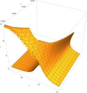 The same plot as a 3D diagram. Varying is shown along a separate axis.
![Frequency response as a function of for the Duffing equation, with and damping The dashed parts of the frequency response are unstable.[3]](/File:Duffing_frequency_response.svg)


![{\displaystyle {\begin{cases}y=\left(\omega ^{2}-\alpha -{\frac {3}{4}}\beta z^{2}\right)^{2}+\left(\delta \omega \right)^{2}\\[1ex]y={\dfrac {\gamma ^{2}}{z^{2}}}\end{cases}}}](https://wikimedia.org/api/rest_v1/media/math/render/svg/cbd3ec81bede4767074dbc99db1ee9a33b5e7abc)


