Exponential distribution

Exponential

Probability density function
Cumulative distribution function
Parameters	${\displaystyle \lambda >0,}$ rate, or inverse scale
Support	${\displaystyle x\in [0,\infty )}$
PDF	${\displaystyle \lambda e^{-\lambda x}}$
CDF	${\displaystyle 1-e^{-\lambda x}}$
Quantile	${\displaystyle -{\frac {\ln(1-p)}{\lambda }}}$
Mean	${\displaystyle {\frac {1}{\lambda }}}$
Median	${\displaystyle {\frac {\ln 2}{\lambda }}}$
Mode	${\displaystyle 0}$
Variance	${\displaystyle {\frac {1}{\lambda ^{2}}}}$
Skewness	${\displaystyle 2}$
Excess kurtosis	${\displaystyle 6}$
Entropy	${\displaystyle 1-\ln \lambda }$
MGF	${\displaystyle {\frac {\lambda }{\lambda -t}},{\text{ for }}t<\lambda }$
CF	${\displaystyle {\frac {\lambda }{\lambda -it}}}$
Fisher information	${\displaystyle {\frac {1}{\lambda ^{2}}}}$
Kullback–Leibler divergence	${\displaystyle \ln {\frac {\lambda _{0}}{\lambda }}+{\frac {\lambda }{\lambda _{0}}}-1}$
Expected shortfall	${\displaystyle -{\frac {\ln(1-p)+1}{\lambda }}}$

In

. In addition to being used for the analysis of Poisson point processes it is found in various other contexts.

The exponential distribution is not the same as the class of exponential families of distributions. This is a large class of probability distributions that includes the exponential distribution as one of its members, but also includes many other distributions, like the normal, binomial, gamma, and Poisson distributions.

Definitions

Probability density function

The probability density function (pdf) of an exponential distribution is

${\displaystyle f(x;\lambda )={\begin{cases}\lambda e^{-\lambda x}&x\geq 0,\\0&x<0.\end{cases}}}$

Here λ > 0 is the parameter of the distribution, often called the rate parameter. The distribution is supported on the interval [0, ∞). If a random variable X has this distribution, we write X ~ Exp(λ).

The exponential distribution exhibits infinite divisibility.

Cumulative distribution function

The cumulative distribution function is given by

${\displaystyle F(x;\lambda )={\begin{cases}1-e^{-\lambda x}&x\geq 0,\\0&x<0.\end{cases}}}$

Alternative parametrization

The exponential distribution is sometimes parametrized in terms of the scale parameter β = 1/λ, which is also the mean:

Properties

Mean, variance, moments, and median

first moment

.

preimage

F⁻¹(1/2).

The mean or expected value of an exponentially distributed random variable X with rate parameter λ is given by

In light of the examples given below, this makes sense; a person who receives an average of two telephone calls per hour can expect that the time between consecutive calls will be 0.5 hour, or 30 minutes.

The variance of X is given by

so the standard deviation is equal to the mean.

The moments of X, for ${\displaystyle n\in \mathbb {N} }$ are given by

The central moments of X, for ${\displaystyle n\in \mathbb {N} }$ are given by

where !n is the subfactorial of n

The median of X is given by

where ln refers to the natural logarithm. Thus the absolute difference between the mean and median is

in accordance with the median-mean inequality.

Memorylessness property of exponential random variable

An exponentially distributed random variable T obeys the relation

This can be seen by considering the complementary cumulative distribution function:

When T is interpreted as the waiting time for an event to occur relative to some initial time, this relation implies that, if T is conditioned on a failure to observe the event over some initial period of time s, the distribution of the remaining waiting time is the same as the original unconditional distribution. For example, if an event has not occurred after 30 seconds, the conditional probability that occurrence will take at least 10 more seconds is equal to the unconditional probability of observing the event more than 10 seconds after the initial time.

The exponential distribution and the geometric distribution are the only memoryless probability distributions.

The exponential distribution is consequently also necessarily the only continuous probability distribution that has a constant failure rate.

Quantiles

The quantile function (inverse cumulative distribution function) for Exp(λ) is

The quartiles are therefore:

• first quartile: ln(4/3)/λ
• median: ln(2)/λ
• third quartile: ln(4)/λ

And as a consequence the interquartile range is ln(3)/λ.

Conditional Value at Risk (Expected Shortfall)

The conditional value at risk (CVaR) also known as the expected shortfall or superquantile for Exp(λ) is derived as follows:^[1]

Buffered Probability of Exceedance (bPOE)

The buffered probability of exceedance is one minus the probability level at which the CVaR equals the threshold ${\displaystyle x}$. It is derived as follows:^[1]

Kullback–Leibler divergence

The directed Kullback–Leibler divergence in nats of ${\displaystyle e^{\lambda }}$ ("approximating" distribution) from ${\displaystyle e^{\lambda _{0}}}$ ('true' distribution) is given by

Maximum entropy distribution

Among all continuous probability distributions with support [0, ∞) and mean μ, the exponential distribution with λ = 1/μ has the largest differential entropy. In other words, it is the maximum entropy probability distribution for a random variate X which is greater than or equal to zero and for which E[X] is fixed.^[2]

Distribution of the minimum of exponential random variables

Let X₁, …, X_n be

exponentially distributed random variables with rate parameters λ₁, …, λ_n. Then is also exponentially distributed, with parameter

This can be seen by considering the complementary cumulative distribution function:

The index of the variable which achieves the minimum is distributed according to the categorical distribution

A proof can be seen by letting ${\displaystyle I=\operatorname {argmin} _{i\in \{1,\dotsb ,n\}}\{X_{1},\dotsc ,X_{n}\}}$. Then,

Note that

is not exponentially distributed, if X₁, …, X_n do not all have parameter 0.^[3]

Joint moments of i.i.d. exponential order statistics

Let ${\displaystyle X_{1},\dotsc ,X_{n}}$ be ${\displaystyle n}$ independent and identically distributed exponential random variables with rate parameter λ. Let ${\displaystyle X_{(1)},\dotsc ,X_{(n)}}$ denote the corresponding order statistics. For ${\displaystyle i<j}$ , the joint moment ${\displaystyle \operatorname {E} \left[X_{(i)}X_{(j)}\right]}$ of the order statistics ${\displaystyle X_{(i)}}$ and ${\displaystyle X_{(j)}}$ is given by

This can be seen by invoking the law of total expectation and the memoryless property:

The first equation follows from the law of total expectation. The second equation exploits the fact that once we condition on ${\displaystyle X_{(i)}=x}$, it must follow that ${\displaystyle X_{(j)}\geq x}$. The third equation relies on the memoryless property to replace ${\displaystyle \operatorname {E} \left[X_{(j)}\mid X_{(j)}\geq x\right]}$ with ${\displaystyle \operatorname {E} \left[X_{(j)}\right]+x}$.

Sum of two independent exponential random variables

The probability distribution function (PDF) of a sum of two independent random variables is the convolution of their individual PDFs. If ${\displaystyle X_{1}}$ and ${\displaystyle X_{2}}$ are independent exponential random variables with respective rate parameters ${\displaystyle \lambda _{1}}$ and ${\displaystyle \lambda _{2},}$ then the probability density of ${\displaystyle Z=X_{1}+X_{2}}$ is given by

The entropy of this distribution is available in closed form: assuming ${\displaystyle \lambda _{1}>\lambda _{2}}$ (without loss of generality), then where ${\displaystyle \gamma }$ is the , and ${\displaystyle \psi (\cdot )}$ is the digamma function.^[4]

In the case of equal rate parameters, the result is an Erlang distribution with shape 2 and parameter ${\displaystyle \lambda ,}$ which in turn is a special case of gamma distribution.

The sum of n independent Exp(λ) exponential random variables is Gamma(n, λ) gamma distributed.

Related distributions

This section includes a list of general references, but it lacks sufficient corresponding inline citations. Please help to improve this section by introducing more precise citations. (March 2011) (Learn how and when to remove this template message)

• If X ~ Laplace(μ, β⁻¹), then |X − μ| ~ Exp(β).
• If X ~ Pareto(1, λ), then log(X) ~ Exp(λ).
• If X ~
  SkewLogistic(θ)
  , then ${\displaystyle \log \left(1+e^{-X}\right)\sim \operatorname {Exp} (\theta )}$.
• If X_i ~
  U(0, 1)
  then
  $${\displaystyle \lim _{n\to \infty }n\min \left(X_{1},\ldots ,X_{n}\right)\sim \operatorname {Exp} (1)}$$

  
• The exponential distribution is a limit of a scaled beta distribution:
  $${\displaystyle \lim _{n\to \infty }n\operatorname {Beta} (1,n)=\operatorname {Exp} (1).}$$

  
• Exponential distribution is a special case of type 3 Pearson distribution.
• If X ~ Exp(λ) and X_i ~ Exp(λ_i) then:
  • ${\displaystyle kX\sim \operatorname {Exp} \left({\frac {\lambda }{k}}\right)}$, closure under scaling by a positive factor.
  • 1 + X ~
    BenktanderWeibull
    (λ, 1), which reduces to a truncated exponential distribution.
  • ke^X ~ Pareto(k, λ).
  • e^−X ~ Beta(λ, 1).
  • 1/ke^X ~ PowerLaw(k, λ)
  • ${\displaystyle {\sqrt {X}}\sim \operatorname {Rayleigh} \left({\frac {1}{\sqrt {2\lambda }}}\right)}$, the Rayleigh distribution
  • ${\displaystyle X\sim \operatorname {Weibull} \left({\frac {1}{\lambda }},1\right)}$, the Weibull distribution
  • ${\displaystyle X^{2}\sim \operatorname {Weibull} \left({\frac {1}{\lambda ^{2}}},{\frac {1}{2}}\right)}$
  • μ − β log(λX) ∼ Gumbel(μ, β).
  • ${\displaystyle \lfloor X\rfloor \sim \operatorname {Geometric} \left(1-e^{-\lambda }\right)}$, a geometric distribution on 0,1,2,3,...
  • ${\displaystyle \lceil X\rceil \sim \operatorname {Geometric} \left(1-e^{-\lambda }\right)}$, a geometric distribution on 1,2,3,4,...
  • If also Y ~ Erlang(n, λ) or${\displaystyle Y\sim \Gamma \left(n,{\frac {1}{\lambda }}\right)}$ then ${\displaystyle {\frac {X}{Y}}+1\sim \operatorname {Pareto} (1,n)}$
  • If also λ ~
    mixture
  • λ₁X₁ − λ₂Y₂ ~ Laplace(0, 1).
  • min{X₁, ..., X_n} ~ Exp(λ₁ + ... + λ_n).
  • If also λ_i = λ then:
    • ${\displaystyle X_{1}+\cdots +X_{k}=\sum _{i}X_{i}\sim }$ Erlang(k, λ) = Gamma(k, λ⁻¹) = Gamma(k, λ) (in (k, θ) and (α, β) parametrization, respectively) with an integer shape parameter k.^[5]
    • If ${\displaystyle T=(X_{1}+\cdots +X_{n})=\sum _{i=1}^{n}X_{i}}$, then ${\displaystyle 2\lambda T\sim \chi _{2n}^{2}}$.
    • X_i − X_j ~ Laplace(0, λ⁻¹).
  • If also X_i are independent, then:
    • ${\displaystyle {\frac {X_{i}}{X_{i}+X_{j}}}}$ ~
      U
      (0, 1)
    • ${\displaystyle Z={\frac {\lambda _{i}X_{i}}{\lambda _{j}X_{j}}}}$ has probability density function ${\displaystyle f_{Z}(z)={\frac {1}{(z+1)^{2}}}}$. This can be used to obtain a confidence interval for ${\displaystyle {\frac {\lambda _{i}}{\lambda _{j}}}}$.
  • If also λ = 1:
    • ${\displaystyle \mu -\beta \log \left({\frac {e^{-X}}{1-e^{-X}}}\right)\sim \operatorname {Logistic} (\mu ,\beta )}$, the logistic distribution
    • ${\displaystyle \mu -\beta \log \left({\frac {X_{i}}{X_{j}}}\right)\sim \operatorname {Logistic} (\mu ,\beta )}$
    • μ − σ log(X) ~ GEV(μ, σ, 0).
    • Further if ${\displaystyle Y\sim \Gamma \left(\alpha ,{\frac {\beta }{\alpha }}\right)}$ then ${\displaystyle {\sqrt {XY}}\sim \operatorname {K} (\alpha ,\beta )}$ (K-distribution)
  • If also λ = 1/2 then X ∼ χ²
    ₂; i.e., X has a chi-squared distribution with 2 degrees of freedom. Hence:
    $${\displaystyle \operatorname {Exp} (\lambda )={\frac {1}{2\lambda }}\operatorname {Exp} \left({\frac {1}{2}}\right)\sim {\frac {1}{2\lambda }}\chi _{2}^{2}\Rightarrow \sum _{i=1}^{n}\operatorname {Exp} (\lambda )\sim {\frac {1}{2\lambda }}\chi _{2n}^{2}}$$

    
• If ${\displaystyle X\sim \operatorname {Exp} \left({\frac {1}{\lambda }}\right)}$ and ${\displaystyle Y\mid X}$ ~ Poisson(X) then ${\displaystyle Y\sim \operatorname {Geometric} \left({\frac {1}{1+\lambda }}\right)}$ (geometric distribution)
• The
  Hoyt distribution can be obtained from exponential distribution and arcsine distribution
• The exponential distribution is a limit of the
  κ-exponential distribution
  in the ${\displaystyle \kappa =0}$ case.
• Exponential distribution is a limit of the κ-Generalized Gamma distribution in the ${\displaystyle \alpha =1}$ and ${\displaystyle \nu =1}$ cases:

  ${\displaystyle \lim _{(\alpha ,\nu )\to (0,1)}p_{\kappa }(x)=(1+\kappa \nu )(2\kappa )^{\nu }{\frac {\Gamma {\Big (}{\frac {1}{2\kappa }}+{\frac {\nu }{2}}{\Big )}}{\Gamma {\Big (}{\frac {1}{2\kappa }}-{\frac {\nu }{2}}{\Big )}}}{\frac {\alpha \lambda ^{\nu }}{\Gamma (\nu )}}x^{\alpha \nu -1}\exp _{\kappa }(-\lambda x^{\alpha })=\lambda e^{-\lambda x}}$

Other related distributions:

• Hyper-exponential distribution
  – the distribution whose density is a weighted sum of exponential densities.
• Hypoexponential distribution – the distribution of a general sum of exponential random variables.
• exGaussian distribution – the sum of an exponential distribution and a normal distribution
  .

Statistical inference

Below, suppose random variable X is exponentially distributed with rate parameter λ, and ${\displaystyle x_{1},\dotsc ,x_{n}}$ are n independent samples from X, with sample mean ${\displaystyle {\bar {x}}}$.

Parameter estimation

The

maximum likelihood

estimator for λ is constructed as follows.

The

independent and identically distributed

sample x = (x₁, …, x_n) drawn from the variable, is:

$${\displaystyle L(\lambda )=\prod _{i=1}^{n}\lambda \exp(-\lambda x_{i})=\lambda ^{n}\exp \left(-\lambda \sum _{i=1}^{n}x_{i}\right)=\lambda ^{n}\exp \left(-\lambda n{\overline {x}}\right),}$$

where:

$${\displaystyle {\overline {x}}={\frac {1}{n}}\sum _{i=1}^{n}x_{i}}$$

is the sample mean.

The derivative of the likelihood function's logarithm is:

$${\displaystyle {\frac {d}{d\lambda }}\ln L(\lambda )={\frac {d}{d\lambda }}\left(n\ln \lambda -\lambda n{\overline {x}}\right)={\frac {n}{\lambda }}-n{\overline {x}}\ {\begin{cases}>0,&0<\lambda <{\frac {1}{\overline {x}}},\\[8pt]=0,&\lambda ={\frac {1}{\overline {x}}},\\[8pt]<0,&\lambda >{\frac {1}{\overline {x}}}.\end{cases}}}$$

Consequently, the

maximum likelihood

estimate for the rate parameter is:

$${\displaystyle {\widehat {\lambda }}_{\text{mle}}={\frac {1}{\overline {x}}}={\frac {n}{\sum _{i}x_{i}}}}$$

This is not an

unbiased estimator

of ${\displaystyle \lambda ,}$ although ${\displaystyle {\overline {x}}}$ is an unbiased[6] MLE^[7] estimator of ${\displaystyle 1/\lambda }$ and the distribution mean.

The bias of ${\displaystyle {\widehat {\lambda }}_{\text{mle}}}$ is equal to

which yields the bias-corrected maximum likelihood estimator

An approximate minimizer of mean squared error (see also: bias–variance tradeoff) can be found, assuming a sample size greater than two, with a correction factor to the MLE:

This is derived from the mean and variance of the inverse-gamma distribution, ${\textstyle {\mbox{Inv-Gamma}}(n,\lambda )}$.^[8]

Fisher information

The Fisher information, denoted ${\displaystyle {\mathcal {I}}(\lambda )}$, for an estimator of the rate parameter ${\displaystyle \lambda }$ is given as:

Plugging in the distribution and solving gives:

This determines the amount of information each independent sample of an exponential distribution carries about the unknown rate parameter ${\displaystyle \lambda }$.

Confidence intervals

The 100(1 − α)% confidence interval for the rate parameter of an exponential distribution is given by:^[9]

which is also equal to: where χ²
_p,v is the 100(p) , n is the number of observations of inter-arrival times in the sample, and x-bar is the sample average. A simple approximation to the exact interval endpoints can be derived using a normal approximation to the χ²
_p,v distribution. This approximation gives the following values for a 95% confidence interval:

$${\displaystyle {\begin{aligned}\lambda _{\text{lower}}&={\widehat {\lambda }}\left(1-{\frac {1.96}{\sqrt {n}}}\right)\\\lambda _{\text{upper}}&={\widehat {\lambda }}\left(1+{\frac {1.96}{\sqrt {n}}}\right)\end{aligned}}}$$

This approximation may be acceptable for samples containing at least 15 to 20 elements.[10]

Bayesian inference

The conjugate prior for the exponential distribution is the gamma distribution (of which the exponential distribution is a special case). The following parameterization of the gamma probability density function is useful:

The

p can then be expressed in terms of the likelihood function defined above and a gamma prior:

Now the posterior density p has been specified up to a missing normalizing constant. Since it has the form of a gamma pdf, this can easily be filled in, and one obtains:

Here the hyperparameter α can be interpreted as the number of prior observations, and β as the sum of the prior observations. The posterior mean here is:

Occurrence and applications

Occurrence of events

The exponential distribution occurs naturally when describing the lengths of the inter-arrival times in a homogeneous

.

The exponential distribution may be viewed as a continuous counterpart of the geometric distribution, which describes the number of Bernoulli trials necessary for a discrete process to change state. In contrast, the exponential distribution describes the time for a continuous process to change state.

In real-world scenarios, the assumption of a constant rate (or probability per unit time) is rarely satisfied. For example, the rate of incoming phone calls differs according to the time of day. But if we focus on a time interval during which the rate is roughly constant, such as from 2 to 4 p.m. during work days, the exponential distribution can be used as a good approximate model for the time until the next phone call arrives. Similar caveats apply to the following examples which yield approximately exponentially distributed variables:

• The time until a radioactive particle decays, or the time between clicks of a Geiger counter
• The time between receiving one telephone call and the next
• The time until default (on payment to company debt holders) in reduced-form credit risk modeling

Exponential variables can also be used to model situations where certain events occur with a constant probability per unit length, such as the distance between mutations on a DNA strand, or between roadkills on a given road.

In

(which is the distribution of the sum of several independent exponentially distributed variables). in a reliability model. The exponential distribution is however not appropriate to model the overall lifetime of organisms or technical devices, because the "failure rates" here are not constant: more failures occur for very young and for very old systems.

In physics, if you observe a gas at a fixed temperature and pressure in a uniform gravitational field, the heights of the various molecules also follow an approximate exponential distribution, known as the Barometric formula. This is a consequence of the entropy property mentioned below.

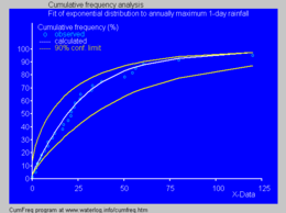
In hydrology, the exponential distribution is used to analyze extreme values of such variables as monthly and annual maximum values of daily rainfall and river discharge volumes.^[12]

The blue picture illustrates an example of fitting the exponential distribution to ranked annually maximum one-day rainfalls showing also the 90%

plotting positions as part of the cumulative frequency analysis

.

In operating-rooms management, the distribution of surgery duration for a category of surgeries with no typical work-content (like in an emergency room, encompassing all types of surgeries).

Prediction

Having observed a sample of n data points from an unknown exponential distribution a common task is to use these samples to make predictions about future data from the same source. A common predictive distribution over future samples is the so-called plug-in distribution, formed by plugging a suitable estimate for the rate parameter λ into the exponential density function. A common choice of estimate is the one provided by the principle of maximum likelihood, and using this yields the predictive density over a future sample x_n+1, conditioned on the observed samples x = (x₁, ..., x_n) given by

The Bayesian approach provides a predictive distribution which takes into account the uncertainty of the estimated parameter, although this may depend crucially on the choice of prior.

A predictive distribution free of the issues of choosing priors that arise under the subjective Bayesian approach is

which can be considered as

1. a frequentist confidence distribution, obtained from the distribution of the pivotal quantity ${\displaystyle {x_{n+1}}/{\overline {x}}}$;^[13]
2. a profile predictive likelihood, obtained by eliminating the parameter λ from the joint likelihood of x_n+1 and λ by maximization;^[14]
3. an objective Bayesian predictive posterior distribution, obtained using the non-informative Jeffreys prior 1/λ;
4. the Conditional Normalized Maximum Likelihood (CNML) predictive distribution, from information theoretic considerations.^[15]

The accuracy of a predictive distribution may be measured using the distance or divergence between the true exponential distribution with rate parameter, λ₀, and the predictive distribution based on the sample x. The Kullback–Leibler divergence is a commonly used, parameterisation free measure of the difference between two distributions. Letting Δ(λ₀||p) denote the Kullback–Leibler divergence between an exponential with rate parameter λ₀ and a predictive distribution p it can be shown that

where the expectation is taken with respect to the exponential distribution with rate parameter λ₀ ∈ (0, ∞), and ψ( · ) is the digamma function. It is clear that the CNML predictive distribution is strictly superior to the maximum likelihood plug-in distribution in terms of average Kullback–Leibler divergence for all sample sizes n > 0.

Random variate generation

A conceptually very simple method for generating exponential

on the unit interval (0, 1), the variate

has an exponential distribution, where F⁻¹ is the quantile function, defined by

Moreover, if U is uniform on (0, 1), then so is 1 − U. This means one can generate exponential variates as follows:

Other methods for generating exponential variates are discussed by Knuth^[16] and Devroye.^[17]

A fast method for generating a set of ready-ordered exponential variates without using a sorting routine is also available.^[17]

See also

• Dead time – an application of exponential distribution to particle detector analysis.
• Laplace distribution, or the "double exponential distribution".
• Relationships among probability distributions
• Marshall–Olkin exponential distribution

References

External links

• "Exponential distribution", Encyclopedia of Mathematics, EMS Press, 2001 [1994]
• Online calculator of Exponential Distribution

References

- ^ "7.2: Exponential Distribution". Statistics LibreTexts. 2021-07-15. Retrieved 2024-10-11.
- ^ "Exponential distribution | mathematics | Britannica". www.britannica.com. Retrieved 2024-10-11.
- ^ a b Weisstein, Eric W. "Exponential Distribution". mathworld.wolfram.com. Retrieved 2024-10-11.
- ^ doi:10.1007/s10479-019-03373-1. Archived from the original(PDF) on 2023-03-31. Retrieved 2023-02-27.
- doi:10.1016/j.jeconom.2008.12.014. Archived from the original(PDF) on 2016-03-07. Retrieved 2011-06-02.
- ^ Michael, Lugo. "The expectation of the maximum of exponentials" (PDF). Archived from the original (PDF) on 20 December 2016. Retrieved 13 December 2016.
- arXiv:1609.02911 [cs.IT].
- ^ .
- ISBN 9780128010358.
- ISBN 978-0-13-187715-3. Retrieved 10 August 2012.
- ^ NIST/SEMATECH e-Handbook of Statistical Methods
- .
- ISBN 978-0-12-370483-2.
- ^ Guerriero, V. (2012). "Power Law Distribution: Method of Multi-scale Inferential Statistics". Journal of Modern Mathematics Frontier. 1: 21–28.
- ^ "Cumfreq, a free computer program for cumulative frequency analysis".
- ISBN 90-70754-33-9.
- ISBN 0-201-89684-2. See section 3.4.1, p. 133.
- ^ ISBN 0-387-96305-7. See chapter IX, section 2, pp. 392–401.