Vorticity

Part of a series on
Continuum mechanics
${\displaystyle J=-D{\frac {d\varphi }{dx}}}$ Fick's laws of diffusion
Laws Conservations Mass Momentum Energy Inequalities Clausius–Duhem (entropy)
Solid mechanics Deformation Elasticity linear Plasticity Hooke's law Stress Strain Finite strain Infinitesimal strain Compatibility Bending Contact mechanics frictional Material failure theory Fracture mechanics
Fluid mechanics Fluids Statics · Dynamics Archimedes' principle · Bernoulli's principle Navier–Stokes equations Poiseuille equation · Pascal's law Viscosity (Newtonian · non-Newtonian) Buoyancy · Mixing · Pressure Liquids Adhesion Capillary action Chromatography Cohesion (chemistry) Surface tension Gases Atmosphere Boyle's law Charles's law Combined gas law Fick's law Gay-Lussac's law Graham's law Plasma
Rheology Viscoelasticity Rheometry Rheometer Smart fluids Electrorheological Magnetorheological Ferrofluids
Scientists Bernoulli Boyle Cauchy Charles Euler Fick Gay-Lussac Graham Hooke Newton Navier Noll Pascal Stokes Truesdell
v t e

In

Mathematically, the vorticity ${\displaystyle {\vec {\omega }}}$ is the curl of the flow velocity ${\displaystyle {\vec {u}}}$:^[4][3]

${\displaystyle {\vec {\omega }}\equiv \nabla \times {\vec {u}}\,,}$

where ${\displaystyle \nabla }$ is the

. Conceptually, ${\displaystyle {\vec {\omega }}}$ could be determined by marking parts of a continuum in a small neighborhood of the point in question, and watching their relative displacements as they move along the flow. The vorticity ${\displaystyle {\vec {\omega }}}$ would be twice the mean angular velocity vector of those particles relative to their center of mass, oriented according to the right-hand rule.

In a two-dimensional flow, ${\displaystyle {\vec {\omega }}}$ is always perpendicular to the plane of the flow, and can therefore be considered a scalar field.

Examples

In a mass of continuum that is rotating like a rigid body, the vorticity is twice the angular velocity vector of that rotation. This is the case, for example, in the central core of a Rankine vortex.^[5]

The vorticity may be nonzero even when all particles are flowing along straight and parallel

, all particles travel parallel to the axis of the pipe; but faster near that axis, and practically stationary next to the walls. The vorticity will be zero on the axis, and maximum near the walls, where the shear is largest.

Conversely, a flow may have zero vorticity even though its particles travel along curved trajectories. An example is the ideal irrotational vortex, where most particles rotate about some straight axis, with speed inversely proportional to their distances to that axis. A small parcel of continuum that does not straddle the axis will be rotated in one sense but sheared in the opposite sense, in such a way that their mean angular velocity about their center of mass is zero.

Example flows:
Rigid-body-like vortex v ∝ r	Parallel flow with shear	Irrotational vortex v ∝ 1/r
where v is the velocity of the flow, r is the distance to the center of the vortex and ∝ indicates proportionality. Absolute velocities around the highlighted point: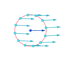
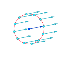
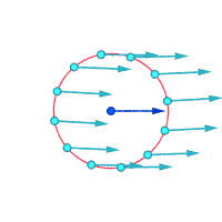
Relative velocities (magnified) around the highlighted point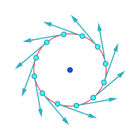
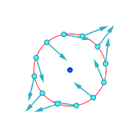
Vorticity ≠ 0	Vorticity ≠ 0	Vorticity = 0

Another way to visualize vorticity is to imagine that, instantaneously, a tiny part of the continuum becomes solid and the rest of the flow disappears. If that tiny new solid particle is rotating, rather than just moving with the flow, then there is vorticity in the flow. In the figure below, the left subfigure demonstrates no vorticity, and the right subfigure demonstrates existence of vorticity.

Mathematical definition

Mathematically, the vorticity of a three-dimensional flow is a pseudovector field, usually denoted by ${\displaystyle {\vec {\omega }}}$, defined as the curl of the velocity field ${\displaystyle {\vec {v}}}$ describing the continuum motion. In

:

${\displaystyle {\begin{aligned}{\vec {\omega }}=\nabla \times {\vec {v}}&={\begin{pmatrix}{\dfrac {\partial }{\partial x}}&\,{\dfrac {\partial }{\partial y}}&\,{\dfrac {\partial }{\partial z}}\end{pmatrix}}\times {\begin{pmatrix}v_{x}&v_{y}&v_{z}\end{pmatrix}}\\[6px]&={\begin{pmatrix}{\dfrac {\partial v_{z}}{\partial y}}-{\dfrac {\partial v_{y}}{\partial z}}&\quad {\dfrac {\partial v_{x}}{\partial z}}-{\dfrac {\partial v_{z}}{\partial x}}&\quad {\dfrac {\partial v_{y}}{\partial x}}-{\dfrac {\partial v_{x}}{\partial y}}\end{pmatrix}}\,.\end{aligned}}}$

In words, the vorticity tells how the velocity vector changes when one moves by an infinitesimal distance in a direction perpendicular to it.

In a two-dimensional flow where the velocity is independent of the ${\displaystyle z}$-coordinate and has no ${\displaystyle z}$-component, the vorticity vector is always parallel to the ${\displaystyle z}$-axis, and therefore can be expressed as a scalar field multiplied by a constant unit vector ${\displaystyle {\hat {z}}}$:

${\displaystyle {\begin{aligned}{\vec {\omega }}=\nabla \times {\vec {v}}&={\begin{pmatrix}{\dfrac {\partial }{\partial x}}&\,{\dfrac {\partial }{\partial y}}&\,{\dfrac {\partial }{\partial z}}\end{pmatrix}}\times {\begin{pmatrix}v_{x}&v_{y}&v_{z}\end{pmatrix}}\\[6px]&=\left({\frac {\partial v_{y}}{\partial x}}-{\frac {\partial v_{x}}{\partial y}}\right){\hat {z}}\,.\end{aligned}}}$

The vorticity is also related to the flow's

${\displaystyle {\vec {n}}}$ and area ${\displaystyle dA}$, the circulation ${\displaystyle d\Gamma }$ along the perimeter of ${\displaystyle C}$ is the dot product ${\displaystyle {\vec {\omega }}\cdot ({\vec {n}}\,dA)}$ where ${\displaystyle {\vec {\omega }}}$ is the vorticity at the center of ${\displaystyle C}$.^[6]

Evolution

The evolution of the vorticity field in time is described by the vorticity equation, which can be derived from the Navier–Stokes equations.^[7]

In many real flows where the viscosity can be neglected (more precisely, in flows with high Reynolds number), the vorticity field can be modeled by a collection of discrete vortices, the vorticity being negligible everywhere except in small regions of space surrounding the axes of the vortices. This is true in the case of two-dimensional potential flow (i.e. two-dimensional zero viscosity flow), in which case the flowfield can be modeled as a complex-valued field on the complex plane.

Vorticity is useful for understanding how ideal potential flow solutions can be perturbed to model real flows. In general, the presence of viscosity causes a diffusion of vorticity away from the vortex cores into the general flow field; this flow is accounted for by a diffusion term in the vorticity transport equation.^[8]

Vortex lines and vortex tubes

A vortex line or vorticity line is a line which is everywhere tangent to the local vorticity vector. Vortex lines are defined by the relation^[9]

${\displaystyle {\frac {dx}{\omega _{x}}}={\frac {dy}{\omega _{y}}}={\frac {dz}{\omega _{z}}}\,,}$

where ${\displaystyle {\vec {\omega }}=(\omega _{x},\omega _{y},\omega _{z})}$ is the vorticity vector in

.

A vortex tube is the surface in the continuum formed by all vortex lines passing through a given (reducible) closed curve in the continuum. The 'strength' of a vortex tube (also called vortex flux)^[10] is the integral of the vorticity across a cross-section of the tube, and is the same everywhere along the tube (because vorticity has zero divergence). It is a consequence of Helmholtz's theorems (or equivalently, of Kelvin's circulation theorem) that in an inviscid fluid the 'strength' of the vortex tube is also constant with time. Viscous effects introduce frictional losses and time dependence.^[11]

In a three-dimensional flow, vorticity (as measured by the volume integral of the square of its magnitude) can be intensified when a vortex line is extended — a phenomenon known as vortex stretching.^[12] This phenomenon occurs in the formation of a bathtub vortex in outflowing water, and the build-up of a tornado by rising air currents.

Vorticity meters

Rotating-vane vorticity meter

A rotating-vane vorticity meter was invented by Russian hydraulic engineer A. Ya. Milovich (1874–1958). In 1913 he proposed a cork with four blades attached as a device qualitatively showing the magnitude of the vertical projection of the vorticity and demonstrated a motion-picture photography of the float's motion on the water surface in a model of a river bend.^[13]

Rotating-vane vorticity meters are commonly shown in educational films on continuum mechanics (famous examples include the NCFMF's "Vorticity"^[14] and "Fundamental Principles of Flow" by Iowa Institute of Hydraulic Research^[15]).

Specific sciences

Aeronautics

In

, lift per unit of span is the product of circulation, airspeed, and air density.

Atmospheric sciences

The relative vorticity is the vorticity relative to the Earth induced by the air velocity field. This air velocity field is often modeled as a two-dimensional flow parallel to the ground, so that the relative vorticity vector is generally scalar rotation quantity perpendicular to the ground. Vorticity is positive when – looking down onto the Earth's surface – the wind turns counterclockwise. In the northern hemisphere, positive vorticity is called cyclonic rotation, and negative vorticity is anticyclonic rotation; the nomenclature is reversed in the Southern Hemisphere.

The absolute vorticity is computed from the air velocity relative to an inertial frame, and therefore includes a term due to the Earth's rotation, the

.

The

of air masses in the atmosphere over the timescale of a few days, particularly when viewed on levels of constant entropy.

The

numerical weather forecasting

utilized that equation.

In modern numerical weather forecasting models and general circulation models (GCMs), vorticity may be one of the predicted variables, in which case the corresponding time-dependent equation is a prognostic equation.

Related to the concept of vorticity is the helicity ${\displaystyle H(t)}$, defined as

${\displaystyle H(t)=\int _{V}{\vec {u}}\cdot {\vec {\omega }}\,dV}$

where the integral is over a given volume ${\displaystyle V}$. In atmospheric science, helicity of the air motion is important in forecasting supercells and the potential for tornadic activity.^[16]

See also

• Barotropic vorticity equation
• D'Alembert's paradox
• Enstrophy
• Palinstrophy
• Velocity potential
• Vortex
• Vortex tube
• Vortex stretching
• Horseshoe vortex
• Wingtip vortices

Fluid dynamics

• Biot–Savart law
• Circulation
• Vorticity equations
• Kutta–Joukowski theorem

Atmospheric sciences

• Prognostic equation
• Carl-Gustaf Rossby
• Hans Ertel

References

1. ^ Lecture Notes from University of Washington Archived October 16, 2015, at the Wayback Machine
2. ^ Moffatt, H.K. (2015), "Fluid Dynamics", in Nicholas J. Higham; et al. (eds.), The Princeton Companion to Applied Mathematics, Princeton University Press, pp. 467–476
3. ^
   ISBN 0-19-851746-7
   .
4. ISBN 0-19-859679-0
   .
5. ^ Acheson (1990), p. 15
6. ^ Clancy, L.J., Aerodynamics, Section 7.11
7. ^ Guyon, et al (2001), pp. 289–290
8. ISBN 9780691159027
   .
9. ^ Kundu P and Cohen I. Fluid Mechanics.
10. ^ Introduction to Astrophysical Gas Dynamics Archived June 14, 2011, at the Wayback Machine
11. ^ G.K. Batchelor, An Introduction to Fluid Dynamics (1967), Section 2.6, Cambridge University Press ISBN 0521098173
12. ^ Batchelor, section 5.2
13. Joukovsky N.E. (1914). "On the motion of water at a turn of a river". Matematicheskii Sbornik. 28.. Reprinted in: Collected works. Vol. 4. Moscow; Leningrad. 1937. pp. 193–216, 231–233 (abstract in English).{{cite book}}: CS1 maint: location missing publisher (link
    ) "Professor Milovich's float", as Joukovsky refers this vorticity meter to, is schematically shown in figure on page 196 of Collected works.
14. ^ National Committee for Fluid Mechanics Films Archived October 21, 2016, at the Wayback Machine
15. ^ Films by Hunter Rouse — IIHR — Hydroscience & Engineering Archived April 21, 2016, at the Wayback Machine
16. S2CID 23287311
    .

Bibliography

• ISBN 0-19-859679-0
  .
• Landau, L. D.; Lifshitz, E.M. (1987). Fluid Mechanics (2nd ed.). Elsevier.
  ISBN 978-0-08-057073-0
  .
• Pozrikidis, C. (2011). Introduction to Theoretical and Computational Fluid Dynamics. Oxford University Press.
  ISBN 978-0-19-975207-2
  .
• Guyon, Etienne; Hulin, Jean-Pierre; Petit, Luc; Mitescu, Catalin D. (2001). Physical Hydrodynamics. Oxford University Press.
  ISBN 0-19-851746-7
  .
• ISBN 0-521-66396-2
• Clancy, L.J. (1975), Aerodynamics, Pitman Publishing Limited, London
  ISBN 0-273-01120-0
• "Weather Glossary"' The Weather Channel Interactive, Inc.. 2004.
• "Vorticity". Integrated Publishing.

Further reading

• Ohkitani, K., "Elementary Account Of Vorticity And Related Equations". Cambridge University Press. January 30, 2005.
  ISBN 0-521-81984-9
• ISBN 0-387-94197-5
• ISBN 0-521-63948-4
• ISBN 0-19-854493-6
• Arfken, G., "Mathematical Methods for Physicists", 3rd ed. Academic Press, Orlando, Florida. 1985.
  ISBN 0-12-059820-5

External links

Wikimedia Commons has media related to Vorticity.

• Weisstein, Eric W., "Vorticity". Scienceworld.wolfram.com.
• Doswell III, Charles A., "A Primer on Vorticity for Application in Supercells and Tornadoes". Cooperative Institute for Mesoscale Meteorological Studies, Norman, Oklahoma.
• Cramer, M. S., "Navier–Stokes Equations -- Vorticity Transport Theorems: Introduction". Foundations of Fluid Mechanics.
• Parker, Douglas, "ENVI 2210 – Atmosphere and Ocean Dynamics, 9: Vorticity". School of the Environment, University of Leeds. September 2001.
• UC Berkeley
  .
  • "The vorticity equation: incompressible and barotropic fluids".
  • "Interpretation of the vorticity equation".
  • "Kelvin's vorticity theorem for incompressible or barotropic flow".
• "Spherepack 3.1". (includes a collection of FORTRAN vorticity program)
• "Mesoscale Compressible Community (MC2)^{[permanent dead link]} Real-Time Model Predictions". (Potential vorticity analysis)