
Diffusion MRI
| Diffusion MRI | |
|---|---|
 DTI Color Map | |
| MeSH | D038524 |
Diffusion-weighted magnetic resonance imaging (DWI or DW-MRI) is the use of specific
Introduction
In diffusion weighted imaging (DWI), the intensity of each image element (
Diffusion-weighted images are very useful to diagnose vascular strokes in the brain. It is also used more and more in the staging of
Diffusion tensor imaging (DTI) is important when a tissue—such as the neural
Diffusion Basis Spectrum Imaging (DBSI) further separates DTI signals into discrete anisotropic diffusion tensors and a spectrum of isotropic diffusion tensors to better differentiate sub-voxel cellular structures. For example, anisotropic diffusion tensors correlate to axonal fibers, while low isotropic diffusion tensors correlate to cells and high isotropic diffusion tensors correlate to larger structures (such as the lumen or brain ventricles).[7] DBSI has been shown to differentiate some types of brain tumors and multiple sclerosis with higher specificity and sensitivity than conventional DTI.[8][9][10][11] DBSI has also been useful in determining microstructure properties of the brain.[12]
Traditionally, in diffusion-weighted imaging (DWI), three gradient-directions are applied, sufficient to estimate the trace of the diffusion tensor or 'average diffusivity', a putative measure of edema. Clinically, trace-weighted images have proven to be very useful to diagnose vascular strokes in the brain, by early detection (within a couple of minutes) of the hypoxic edema.[13]
More extended DTI scans derive neural tract directional information from the data using 3D or multidimensional vector algorithms based on six or more gradient directions, sufficient to compute the diffusion tensor. The diffusion tensor model is a rather simple model of the diffusion process, assuming homogeneity and linearity of the diffusion within each image voxel.[13] From the diffusion tensor, diffusion anisotropy measures such as the fractional anisotropy (FA), can be computed. Moreover, the principal direction of the diffusion tensor can be used to infer the white-matter connectivity of the brain (i.e. tractography; trying to see which part of the brain is connected to which other part).
Recently, more advanced models of the diffusion process have been proposed that aim to overcome the weaknesses of the diffusion tensor model. Amongst others, these include q-space imaging [14] and generalized diffusion tensor imaging.
Mechanism
Diffusion imaging is an


To sensitize MRI images to diffusion, the magnetic field strength (B1) is varied linearly by a pulsed field gradient. Since precession is proportional to the magnet strength, the protons begin to precess at different rates, resulting in dispersion of the phase and signal loss. Another gradient pulse is applied in the same magnitude but with opposite direction to refocus or rephase the spins. The refocusing will not be perfect for protons that have moved during the time interval between the pulses, and the signal measured by the MRI machine is reduced. This "field gradient pulse" method was initially devised for NMR by Stejskal and Tanner [16] who derived the reduction in signal due to the application of the pulse gradient related to the amount of diffusion that is occurring through the following equation:
![{\displaystyle {\frac {S(TE)}{S_{0}}}=\exp \left[-\gamma ^{2}G^{2}\delta ^{2}\left(\Delta -{\frac {\delta }{3}}\right)D\right]}](https://wikimedia.org/api/rest_v1/media/math/render/svg/355575bbfbd0924e1f733841cfe4a022aafba8e0)
where is the signal intensity without the diffusion weighting, is the signal with the gradient, is the gyromagnetic ratio, is the strength of the gradient pulse, is the duration of the pulse, is the time between the two pulses, and finally, is the diffusion-coefficient.


In order to localize this signal attenuation to get images of diffusion one has to combine the pulsed magnetic field gradient pulses used for MRI (aimed at localization of the signal, but those gradient pulses are too weak to produce a diffusion related attenuation) with additional "motion-probing" gradient pulses, according to the Stejskal and Tanner method. This combination is not trivial, as cross-terms arise between all gradient pulses. The equation set by Stejskal and Tanner then becomes inaccurate and the signal attenuation must be calculated, either analytically or numerically, integrating all gradient pulses present in the MRI sequence and their interactions. The result quickly becomes very complex given the many pulses present in the MRI sequence, and as a simplification, Le Bihan suggested gathering all the gradient terms in a "b factor" (which depends only on the acquisition parameters) so that the signal attenuation simply becomes:[1]

Also, the diffusion coefficient, , is replaced by an apparent diffusion coefficient, , to indicate that the diffusion process is not free in tissues, but hindered and modulated by many mechanisms (restriction in closed spaces, tortuosity around obstacles, etc.) and that other sources of IntraVoxel Incoherent Motion (IVIM) such as blood flow in small vessels or cerebrospinal fluid in ventricles also contribute to the signal attenuation. At the end, images are "weighted" by the diffusion process: In those diffusion-weighted images (DWI) the signal is more attenuated the faster the diffusion and the larger the b factor is. However, those diffusion-weighted images are still also sensitive to T1 and T2 relaxivity contrast, which can sometimes be confusing. It is possible to calculate "pure" diffusion maps (or more exactly ADC maps where the ADC is the sole source of contrast) by collecting images with at least 2 different values, and , of the b factor according to:


![{\displaystyle \mathrm {ADC} (x,y,z)=\ln[S_{2}(x,y,z)/S_{1}(x,y,z)]/(b_{1}-b_{2})}](https://wikimedia.org/api/rest_v1/media/math/render/svg/c9abbc60b76bb6bec8785ad650ea4693ee645b4e)
Although this ADC concept has been extremely successful, especially for clinical applications, it has been challenged recently, as new, more comprehensive models of diffusion in biological tissues have been introduced. Those models have been made necessary, as diffusion in tissues is not free. In this condition, the ADC seems to depend on the choice of b values (the ADC seems to decrease when using larger b values), as the plot of ln(S/So) is not linear with the b factor, as expected from the above equations. This deviation from a free diffusion behavior is what makes diffusion MRI so successful, as the ADC is very sensitive to changes in tissue microstructure. On the other hand, modeling diffusion in tissues is becoming very complex. Among most popular models are the biexponential model, which assumes the presence of 2 water pools in slow or intermediate exchange [17][18] and the cumulant-expansion (also called Kurtosis) model,[19][20][21] which does not necessarily require the presence of 2 pools.
Diffusion model
Given the concentration and flux , Fick's first law gives a relationship between the flux and the concentration gradient:


where D is the

Putting the two together, we get the diffusion equation:

Magnetization dynamics
With no diffusion present, the change in nuclear

which has terms for precession, T2 relaxation, and T1 relaxation.
In 1956, H.C. Torrey mathematically showed how the Bloch equations for magnetization would change with the addition of diffusion.[22] Torrey modified Bloch's original description of transverse magnetization to include diffusion terms and the application of a spatially varying gradient. Since the magnetization is a vector, there are 3 diffusion equations, one for each dimension. The


where is now the diffusion tensor.

For the simplest case where the diffusion is isotropic the diffusion tensor is a multiple of the identity:

then the Bloch-Torrey equation will have the solution

The exponential term will be referred to as the attenuation . Anisotropic diffusion will have a similar solution for the diffusion tensor, except that what will be measured is the apparent diffusion coefficient (ADC). In general, the attenuation is:


where the terms incorporate the gradient fields , , and .


Grayscale
The standard grayscale of DWI images is to represent increased diffusion restriction as brighter.[23]
ADC image

An apparent diffusion coefficient (ADC) image, or an ADC map, is an MRI image that more specifically shows diffusion than conventional DWI, by eliminating the
Cerebral infarction leads to diffusion restriction, and the difference between images with various DWI weighting will therefore be minor, leading to an ADC image with low signal in the infarcted area.[24] A decreased ADC may be detected minutes after a cerebral infarction.[26] The high signal of infarcted tissue on conventional DWI is a result of its partial T2 weighting.[27]
Diffusion tensor imaging
Diffusion tensor imaging (DTI) is a magnetic resonance imaging technique that enables the measurement of the restricted diffusion of water in tissue in order to produce neural tract images instead of using this data solely for the purpose of assigning contrast or colors to pixels in a cross-sectional image. It also provides useful structural information about muscle—including heart muscle—as well as other tissues such as the prostate.[28]
In DTI, each voxel has one or more pairs of parameters: a rate of diffusion and a preferred direction of diffusion—described in terms of three-dimensional space—for which that parameter is valid. The properties of each voxel of a single DTI image are usually calculated by vector or tensor math from six or more different diffusion weighted acquisitions, each obtained with a different orientation of the diffusion sensitizing gradients. In some methods, hundreds of measurements—each making up a complete image—are made to generate a single resulting calculated image data set. The higher information content of a DTI voxel makes it extremely sensitive to subtle pathology in the brain. In addition the directional information can be exploited at a higher level of structure to select and follow neural tracts through the brain—a process called tractography.[29]
A more precise statement of the image acquisition process is that the image-intensities at each position are attenuated, depending on the strength (b-value) and direction of the so-called magnetic diffusion gradient, as well as on the local microstructure in which the water molecules diffuse. The more attenuated the image is at a given position, the greater diffusion there is in the direction of the diffusion gradient. In order to measure the tissue's complete diffusion profile, one needs to repeat the MR scans, applying different directions (and possibly strengths) of the diffusion gradient for each scan.
Mathematical foundation—tensors
Diffusion MRI relies on the mathematics and physical interpretations of the geometric quantities known as tensors. Only a special case of the general mathematical notion is relevant to imaging, which is based on the concept of a symmetric matrix.[notes 1] Diffusion itself is tensorial, but in many cases the objective is not really about trying to study brain diffusion per se, but rather just trying to take advantage of diffusion anisotropy in white matter for the purpose of finding the orientation of the axons and the magnitude or degree of anisotropy. Tensors have a real, physical existence in a material or tissue so that they do not move when the coordinate system used to describe them is rotated. There are numerous different possible representations of a tensor (of rank 2), but among these, this discussion focuses on the ellipsoid because of its physical relevance to diffusion and because of its historical significance in the development of diffusion anisotropy imaging in MRI.
The following matrix displays the components of the diffusion tensor:

The same matrix of numbers can have a simultaneous second use to describe the shape and orientation of an ellipse and the same matrix of numbers can be used simultaneously in a third way for matrix mathematics to sort out eigenvectors and eigenvalues as explained below.
Physical tensors
The idea of a tensor in physical science evolved from attempts to describe the quantity of physical properties. The first properties they were applied to were those that can be described by a single number, such as temperature. Properties that can be described this way are called scalars; these can be considered tensors of rank 0, or 0th-order tensors. Tensors can also be used to describe quantities that have directionality, such as mechanical force. These quantities require specification of both magnitude and direction, and are often represented with a vector. A three-dimensional vector can be described with three components: its projection on the x, y, and z axes. Vectors of this sort can be considered tensors of rank 1, or 1st-order tensors.
A tensor is often a physical or biophysical property that determines the relationship between two vectors. When a force is applied to an object, movement can result. If the movement is in a single direction, the transformation can be described using a vector—a tensor of rank 1. However, in a tissue, diffusion leads to movement of water molecules along trajectories that proceed along multiple directions over time, leading to a complex projection onto the Cartesian axes. This pattern is reproducible if the same conditions and forces are applied to the same tissue in the same way. If there is an internal anisotropic organization of the tissue that constrains diffusion, then this fact will be reflected in the pattern of diffusion. The relationship between the properties of driving force that generate diffusion of the water molecules and the resulting pattern of their movement in the tissue can be described by a tensor. The collection of molecular displacements of this physical property can be described with nine components—each one associated with a pair of axes xx, yy, zz, xy, yx, xz, zx, yz, zy.[30] These can be written as a matrix similar to the one at the start of this section.
Diffusion from a point source in the anisotropic medium of white matter behaves in a similar fashion. The first pulse of the Stejskal Tanner diffusion gradient effectively labels some water molecules and the second pulse effectively shows their displacement due to diffusion. Each gradient direction applied measures the movement along the direction of that gradient. Six or more gradients are summed to get all the measurements needed to fill in the matrix, assuming it is symmetric above and below the diagonal (red subscripts).
In 1848, Henri Hureau de Sénarmont[31] applied a heated point to a polished crystal surface that had been coated with wax. In some materials that had "isotropic" structure, a ring of melt would spread across the surface in a circle. In anisotropic crystals the spread took the form of an ellipse. In three dimensions this spread is an ellipsoid. As Adolf Fick showed in the 1850s, diffusion exhibits many of the same patterns as those seen in the transfer of heat.
Mathematics of ellipsoids
At this point, it is helpful to consider the mathematics of ellipsoids. An ellipsoid can be described by the formula: . This equation describes a quadric surface. The relative values of a, b, and c determine if the quadric describes an ellipsoid or a hyperboloid.

As it turns out, three more components can be added as follows: . Many combinations of a, b, c, d, e, and f still describe ellipsoids, but the additional components (d, e, f) describe the rotation of the ellipsoid relative to the orthogonal axes of the Cartesian coordinate system. These six variables can be represented by a matrix similar to the tensor matrix defined at the start of this section (since diffusion is symmetric, then we only need six instead of nine components—the components below the diagonal elements of the matrix are the same as the components above the diagonal). This is what is meant when it is stated that the components of a matrix of a second order tensor can be represented by an ellipsoid—if the diffusion values of the six terms of the quadric ellipsoid are placed into the matrix, this generates an ellipsoid angled off the orthogonal grid. Its shape will be more elongated if the relative anisotropy is high.

When the ellipsoid/tensor is represented by a matrix, we can apply a useful technique from standard matrix mathematics and linear algebra—that is to "diagonalize" the matrix. This has two important meanings in imaging. The idea is that there are two equivalent ellipsoids—of identical shape but with different size and orientation. The first one is the measured diffusion ellipsoid sitting at an angle determined by the axons, and the second one is perfectly aligned with the three Cartesian axes. The term "diagonalize" refers to the three components of the matrix along a diagonal from upper left to lower right (the components with red subscripts in the matrix at the start of this section). The variables , , and are along the diagonal (red subscripts), but the variables d, e and f are "off diagonal". It then becomes possible to do a vector processing step in which we rewrite our matrix and replace it with a new matrix multiplied by three different vectors of unit length (length=1.0). The matrix is diagonalized because the off-diagonal components are all now zero. The rotation angles required to get to this equivalent position now appear in the three vectors and can be read out as the x, y, and z components of each of them. Those three vectors are called "


Measures of anisotropy and diffusivity

In present-day clinical neurology, various brain pathologies may be best detected by looking at particular measures of anisotropy and diffusivity. The underlying physical process of diffusion causes a group of water molecules to move out from a central point, and gradually reach the surface of an ellipsoid if the medium is anisotropic (it would be the surface of a sphere for an isotropic medium). The ellipsoid formalism functions also as a mathematical method of organizing tensor data. Measurement of an ellipsoid tensor further permits a retrospective analysis, to gather information about the process of diffusion in each voxel of the tissue.[32]
In an isotropic medium such as
Once we have measured the voxel from six or more directions and corrected for attenuations due to T2 and T1 effects, we can use information from our calculated ellipsoid tensor to describe what is happening in the voxel. If you consider an ellipsoid sitting at an angle in a Cartesian grid then you can consider the projection of that ellipse onto the three axes. The three projections can give you the ADC along each of the three axes ADCx, ADCy, ADCz. This leads to the idea of describing the average diffusivity in the voxel which will simply be

We use the i subscript to signify that this is what the isotropic diffusion coefficient would be with the effects of anisotropy averaged out.
The ellipsoid itself has a principal long axis and then two more small axes that describe its width and depth. All three of these are perpendicular to each other and cross at the center point of the ellipsoid. We call the axes in this setting
The diffusivity along the principal axis, λ1 is also called the longitudinal diffusivity or the axial diffusivity or even the parallel diffusivity λ∥. Historically, this is closest to what Richards originally measured with the vector length in 1991.[33] The diffusivities in the two minor axes are often averaged to produce a measure of radial diffusivity

This quantity is an assessment of the degree of restriction due to membranes and other effects and proves to be a sensitive measure of degenerative pathology in some neurological conditions.[34] It can also be called the perpendicular diffusivity ().

Another commonly used measure that summarizes the total diffusivity is the Trace—which is the sum of the three eigenvalues,

where is a diagonal matrix with eigenvalues , and on its diagonal.


If we divide this sum by three we have the mean diffusivity,

which equals ADCi since

where is the matrix of eigenvectors and is the diffusion tensor. Aside from describing the amount of diffusion, it is often important to describe the relative degree of anisotropy in a voxel. At one extreme would be the sphere of isotropic diffusion and at the other extreme would be a cigar or pencil shaped very thin


![{\displaystyle \mathrm {FA} ={\frac {\sqrt {3((\lambda _{1}-\operatorname {E} [\lambda ])^{2}+(\lambda _{2}-\operatorname {E} [\lambda ])^{2}+(\lambda _{3}-\operatorname {E} [\lambda ])^{2})}}{\sqrt {2(\lambda _{1}^{2}+\lambda _{2}^{2}+\lambda _{3}^{2})}}}}](https://wikimedia.org/api/rest_v1/media/math/render/svg/a6b99560a24b2b57e604ec988e52d9c379b10219)
The fractional anisotropy can also be separated into linear, planar, and spherical measures depending on the "shape" of the diffusion ellipsoid.

For the linear case, where ,


For the planar case, where ,


For the spherical case, where ,


Each measure lies between 0 and 1 and they sum to unity. An additional anisotropy measure can used to describe the deviation from the spherical case:

There are other metrics of anisotropy used, including the relative anisotropy (RA):
![{\displaystyle \mathrm {RA} ={\frac {\sqrt {(\lambda _{1}-\operatorname {E} [\lambda ])^{2}+(\lambda _{2}-\operatorname {E} [\lambda ])^{2}+(\lambda _{3}-\operatorname {E} [\lambda ])^{2}}}{{\sqrt {3}}\operatorname {E} [\lambda ]}}}](https://wikimedia.org/api/rest_v1/media/math/render/svg/9510ba237aa82760cef9a3e17be0f1fcd440f8bb)
and the volume ratio (VR):
![{\displaystyle \mathrm {VR} ={\frac {\lambda _{1}\lambda _{2}\lambda _{3}}{\operatorname {E} [\lambda ]^{3}}}}](https://wikimedia.org/api/rest_v1/media/math/render/svg/dd11dafd0f15f1c16165bc6eec8e95583af05af8)
Applications
This section needs additional citations for verification. (December 2013) |
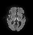
The most common application of conventional DWI (without DTI) is in acute brain ischemia. DWI directly visualizes the ischemic necrosis in cerebral infarction in the form of a cytotoxic edema,[38] appearing as a high DWI signal within minutes of arterial occlusion.[39] With perfusion MRI detecting both the infarcted core and the salvageable penumbra, the latter can be quantified by DWI and perfusion MRI.[40]
-
 DWI showing necrosis (shown as brighter) in a cerebral infarction
 -
 DWI showing restricted diffusion in the medial dorsal thalami consistent with Wernicke encephalopathy
 -
 DWI showing cortical ribbon-like high signal consistent with diffusion restriction in a patient with known MELAS syndrome


Another application area of DWI is in oncology. Tumors are in many instances highly cellular, giving restricted diffusion of water, and therefore appear with a relatively high signal intensity in DWI.[41] DWI is commonly used to detect and stage tumors, and also to monitor tumor response to treatment over time. DWI can also be collected to visualize the whole body using a technique called 'diffusion-weighted whole-body imaging with background body signal suppression' (DWIBS).[42] Some more specialized diffusion MRI techniques such as diffusion kurtosis imaging (DKI) have also been shown to predict the response of cancer patients to chemotherapy treatment.[43]
The principal application is in the imaging of white matter where the location, orientation, and anisotropy of the tracts can be measured. The architecture of the axons in parallel bundles, and their myelin sheaths, facilitate the diffusion of the water molecules preferentially along their main direction. Such preferentially oriented diffusion is called anisotropic diffusion.


The imaging of this property is an extension of diffusion MRI. If a series of diffusion gradients (i.e.
Applications in the brain:
- Tract-specific localization of white matter brain tumors, surgery is aided by knowing the proximity and relative position of the corticospinal tractand a tumor.
- Diffusion tensor imaging data can be used to perform tractography within white matter. Fiber tracking algorithms can be used to track a fiber along its whole length (e.g. the corticospinal tract, through which the motor information transit from the motor cortex to the spinal cord and the peripheral nerves). Tractography is a useful tool for measuring deficits in white matter, such as in aging. Its estimation of fiber orientation and strength is increasingly accurate, and it has widespread potential implications in the fields of cognitive neuroscience and neurobiology.
- The use of DTI for the assessment of white matter in development, pathology and degeneration has been the focus of over 2,500 research publications since 2005. It promises to be very helpful in distinguishing Alzheimer's disease from other types of dementia. Applications in brain research include the investigation of neural networks in vivo, as well as in connectomics.
Applications for peripheral nerves:
- Cubital Tunnel Syndrome: metrics derived from DTI (FA and RD) can differentiate asymptomatic adults from those with compression of the ulnar nerve at the elbow[48]
- Carpal Tunnel Syndrome: Metrics derived from DTI (lower FA and MD) differentiate healthy adults from those with carpal tunnel syndrome[49]
Research
Early in the development of DTI based tractography, a number of researchers pointed out a flaw in the diffusion tensor model. The tensor analysis assumes that there is a single ellipsoid in each imaging voxel—as if all of the axons traveling through a voxel traveled in exactly the same direction.
The Q-Ball method of tractography is an implementation in which David Tuch provides a mathematical alternative to the tensor model.
Note, there is ongoing debate about the best way to preprocess DW-MRI. Several in-vivo studies have shown that the choice of software and functions applied (directed at correcting artefacts from arising from e.g. motion and eddy-currents) have a meaningful impact on the DTI parameter estimates from tissue.[56] Consequently, this is the topic of a multinational study directed by the diffusion-study group of the ISMRM.
Summary
For DTI, it is generally possible to use linear algebra, matrix mathematics and vector mathematics to process the analysis of the tensor data.
In some cases, the full set of tensor properties is of interest, but for tractography it is usually necessary to know only the magnitude and orientation of the primary axis or vector. This primary axis—the one with the greatest length—is the largest eigenvalue and its orientation is encoded in its matched eigenvector. Only one axis is needed as it is assumed the largest eigenvalue is aligned with the main axon direction to accomplish tractography.
See also
Explanatory notes
- component free, and so on, but the generality, which covers arrays of all sizes, may obscure rather than help.
References
- ^ a b Le Bihan, Denis; Breton, E. (1985). "Imagerie de diffusion in-vivo par résonance magnétique nucléaire" [In-vivo diffusion imaging by nuclear magnetic resonance]. Comptes-Rendus de l'Académie des Sciences (in French). 301 (15): 1109–1112. INIST 8814916.
- .
- S2CID 250787827.
- S2CID 8586494.
- S2CID 2660208.
- PMID 3763909.
- PMID 22171354.
- PMID 34132126.
- PMID 32304291.
- PMID 32694155.
- PMID 33637807.
- PMID 34227242.
- ^ .
- S2CID 19766099.
- PMID 8351339.
- .
- S2CID 25910939.
- ISBN 978-0-12-025512-2.
- .
- NAID 10018514722.
- S2CID 11865594.
- .
- ^ a b Elster AD (2021). "Restricted Diffusion". mriquestions.com/. Retrieved 2018-03-15.
- ^ a b Hammer M. "MRI Physics: Diffusion-Weighted Imaging". XRayPhysics. Retrieved 2017-10-15.
- PMID 23882093.
- PMID 21454821.
- ^ Bhuta S. "Diffusion weighted MRI in acute stroke". Radiopaedia. Retrieved 2017-10-15.
- S2CID 14173858.
- PMID 11025519.
- OCLC 576214706.[page needed]
- ^ de Sénarmont HH (1848). "Mémoire sur la conductibilité des substances cristalisées pour la chaleur" [Memoir on the conductivity of crystallized substances for heat]. Comptes Rendus Hebdomadaires des Séances de l'Académie des Sciences (in French). 25: 459–461.
- S2CID 7269302.
- ^ Richards TL, Heide AC, Tsuruda JS, Alvord EC (1992). Vector analysis of diffusion images in experimental allergic encephalomyelitis (PDF). Proceedings of the Society for Magnetic Resonance in Medicine. Vol. 11. Berlin. p. 412.
- PMID 19129507.
- ^ Westin CF, Peled S, Gudbjartsson H, Kikinis R, Jolesz FA (1997). Geometrical diffusion measures for MRI from tensor basis analysis. ISMRM '97. Vancouver Canada. p. 1742.
- PMID 12044998.
- PMID 17599699.
- PMID 23876408.
- ^ Weerakkody Y, Gaillard F, et al. "Ischaemic stroke". Radiopaedia. Retrieved 2017-10-15.
- PMID 22468186.
- PMID 17515386.
- ISBN 978-3-540-78575-0.
- PMID 31341212.
- ^ PMID 32373625.
- S2CID 18718789.
- ^ Soll E (2015). "DTI (Quantitative), a new and advanced MRI procedure for evaluation of Concussions".
- PMID 33282795.
- PMID 34294771.
- PMID 34686721.
- ^ S2CID 1368461.
- NAID 10027851300.
- S2CID 2048187.
- .
- S2CID 6080176.
- S2CID 121103537.
- S2CID 264099038.