
Streeter–Phelps equation

The Streeter–Phelps equation is used in the study of
Streeter–Phelps equation
The Streeter–Phelps equation determines the relation between the

This differential equation states that the total change in oxygen deficit (D) is equal to the difference between the two rates of deoxygenation and reaeration at any time.
The Streeter–Phelps equation, assuming a plug-flow stream at steady state is then


where
- is the saturation deficit, which can be derived from the dissolved oxygen concentration at saturation minus the actual dissolved oxygen concentration (). has the dimensions .
- is the deoxygenation rate, usually in .
- is the reaeration rate, usually in .
- is the initial oxygen demand of organic matter in the water, also called the ultimate BOD (BOD at time t=infinity). The unit of is .
- is the oxygen demand remaining at time t, .
- is the initial oxygen deficit .
- is the elapsed time, usually .


![{\displaystyle [{\tfrac {\mathrm {g} }{\mathrm {m} ^{3}}}]}](https://wikimedia.org/api/rest_v1/media/math/render/svg/1a846316b184fac08cedc66c32bd4ceb071ddaae)

![{\displaystyle [d]}](https://wikimedia.org/api/rest_v1/media/math/render/svg/ef4f4d84e860f2ffd5b55eec14cfbf735dd01689)
lies typically within the range 0.05-0.5 and lies typically within the range 0.4-1.5 .[2]
The Streeter–Phelps equation is also known as the DO sag equation. This is due to the shape of the graph of the DO over time.

Critical oxygen deficit
On the DO sag curve a minimum concentration occurs at some point, along a stream. If the Streeter–Phelps equation is differentiated with respect to time, and set equal to zero, the time at which the minimum DO occurs is expressed by
![{\displaystyle t_{crit}={\frac {1}{k_{2}-k_{1}}}\ln {\left[{\frac {k_{2}}{k_{1}}}\left({1-{\frac {D_{a}(k_{2}-k_{1})}{L_{a}k_{1}}}}\right)\right]}}](https://wikimedia.org/api/rest_v1/media/math/render/svg/fb0a3829bfc0a64c2d3916fd686ed3761aeb1114)
To find the value of the critical oxygen deficit, , the Streeter–Phelps equation is combined with the equation above, for the critical time, . Then the minimum dissolved oxygen concentration is


Mathematically it is possible to get a negative value of , even though it is not possible to have a negative amount of DO in reality.[3]

The distance traveled in a river from a given point source pollution or waste discharge downstream to the (which is the minimum DO) is found by
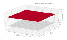
Surface plot depicting the dissolved oxygen (DO) concentration in a river. DO is shown on the vertical axis, with the along-stream and cross-stream directions on the x and y axes, respectively. A continuous input of biological material is added to the river at x = 75 m, y = 15 m, beginning at t = 0.


where is the flow velocity of the stream. This formula is a good approximation as long as the flow can be regarded as a plug flow (turbulent).

Estimation of reaeration rate
Several estimations of the reaeration rate exist, which generally follow the equation

where
- is a constant.
- is the flow velocity [m/s].
- is the depth [m].
- is a constant.
- is a constant.


The constants depend on the system to which the equation is applied, i.e. the flow velocity and the size of the stream or river. Different values are available in the literature.
The software "International Hydrological Programme" applies the following equation derived on the basis of values used in published literature[4]

where
- .
- is the average flow velocity [m/s].
- is the average depth of flow in the river [m].
![{\displaystyle [d^{-1}]}](https://wikimedia.org/api/rest_v1/media/math/render/svg/70f7a7f8b6420c8da2a11bd52e64c99a5c68aef1)
Temperature correction
Both the deoxygenation rate, and reaeration rate, can be temperature corrected, following the general formula.[2]

where
- is the rate at 20 degrees Celsius.
- θ is a constant, which differs for the two rates.
- is the actual temperature in the stream in degC.


Normally θ has the value 1.048 for and 1.024 for . An increasing temperature has the most impact on the deoxygenation rate, and results in an increased critical deficit (), and decreases. Furthermore, a decreased concentration occurs with increasing temperature, which leads to a decrease in the DO concentration.[2]


Mixing of rivers
When two streams or rivers merge or water is discharged to a stream it is possible to determine the BOD and DO after mixing assuming steady state conditions and instantaneous mixing. The two streams are considered as dilutions of each other thus the initial BOD and DO will be [4]

and

where
- is the initial concentration of BOD in the river downstream of the mixing, also called BOD(0). The unit of is .
- is the background BOD of the concentration in the river .
- is the BOD of the content of the merging river .
- is the initial concentration of the dissolved oxygen in the river downstream of the conjoining point .
- is the background concentration of the dissolved oxygen content in the river .
- is the background concentration of the dissolved oxygen content in the merging river .
- is the flow in the river upstream from the mixing point .
- is the flow in the merging river upstream from the mixing point .


![{\displaystyle [{\tfrac {m^{3}}{s}}]}](https://wikimedia.org/api/rest_v1/media/math/render/svg/6e1c4d695d346d5825d718a419c5f822231758ed)

Numerical approach
Nowadays it is possible to solve the classical Streeter–Phelps equation numerically by use of computers. The differential equations are solved by integration.
History
In 1925, a study on the phenomena of oxidation and reaeration in the Ohio River in the US was published by the sanitary engineer, Harold Warner Streeter and the consultant, Earle Bernard Phelps (1876–1953). The study was based on data obtained from May 1914 to April 1915 by the United States Public Health Service under supervision of Surg. W.H. Frost.[1]
More complex versions of the Streeter–Phelps model were introduced during the 1960s, where computers made it possible to include further contributions to the oxygen development in streams. At the head of this development were O'Connor (1960) and Thomann (1963).[5] O'Connor added the contributions from photosynthesis, respiration and sediment oxygen demand (SOD).[6] Thomann expanded the Streeter–Phelps model to allow for multi segment systems.[7]
Applications and limitations
The simple Streeter–Phelps model is based on the assumptions that a single BOD input is distributed evenly at the cross section of a stream or river and that it moves as plug flow with no mixing in the river.[8] Furthermore, only one DO sink (carbonaceous BOD) and one DO source (reaeration) is considered in the classical Streeter–Phelps model.[9] These simplifications will give rise to errors in the model. For example the model does not include BOD removal by sedimentation, that suspended BOD is converted to a dissolved state, that sediment has an oxygen demand and that photosynthesis and respiration will impact the oxygen balance.[8]
Expanded model
In addition to the oxidation of organic matter and the reaeration process, there are many other processes in a stream which affect the DO.[8] In order to make a more accurate model it is possible to include these factors using an expanded model.
The expanded model is a modification of the traditional model and includes internal sources (reaeration and photosynthesis) and sinks (BOD, background BOD, SOD and respiration) of DO. It is not always necessary to include all of these parameters. Instead relevant sources and sinks can be summed to yield the overall solution for the particular model.[2] Parameters in the expanded model can be either measured in the field or estimated theoretically.
Background BOD
Background BOD or benthic oxygen demand is the diffuse source of BOD represented by the decay of organic matter that has already settled on the bottom. This will give rise to a constant diffuse input thus the change in BOD over time will be

where
- is the rate for oxygen consumption by BOD, usually in .
- is the BOD from organic matter in the water .
- is the background BOD input .

Sedimentation of BOD
Sedimented BOD does not directly consume oxygen and this should therefore be taken into account. This is done by introducing a rate of BOD removal combined with a rate of oxygen consumption by BOD. Giving a total rate for oxygen removal by BOD [2]

where
- is the rate of oxygen consumption by BOD, usually in .
- is the rate of settling of BOD, usually in .

The change in BOD over time is described as

where is the BOD from organic matter in the water .
is typically in the range of 0.5-5 .[2]

Sediment oxygen demand

Oxygen can be consumed by organisms in the sediment. This process is referred to as sediment oxygen demand (SOD). Measurement of SOD can be undertaken by measuring the change of oxygen in a box on the sediment (benthic respirometer).
The change in oxygen deficit due to consumption by sediment is described as

where
- is the depth of the river [m]
- is the SOD
- D is the saturation deficit .
- is the reaeration rate [].

![{\displaystyle [{\tfrac {g}{m^{2}d}}]}](https://wikimedia.org/api/rest_v1/media/math/render/svg/c3e7fa46a186240ccb9e63217dddcc2dc3b05404)
The range of the SOD is typically in the range of 0.1 – 1 for a natural river with low pollution and 5 – 10 for a river with moderate to heavy pollution.[2]

Nitrification
Ammonium is oxidized to nitrate under aerobic conditions
- NH4+ + 2O2 → NO3− + H2O + 2H+
Ammonium oxidation can be treated as part of BOD, so that BOD = CBOD + NBOD, where CBOD is the

where
- D is the saturation deficit.
- is the nitrification rate .
- is ammonium-nitrogen concentration.


The range of is typically 0.05-0.5 .[2]
Photosynthesis and respiration
Photosynthesis and respiration are performed by algae and by macrophytes. Respiration is also performed by bacteria and animals. Assuming steady state (net daily average) the change in deficit will be

where
- is the respiration .
- is the photosynthesis .

![{\displaystyle [{\tfrac {mg}{Ld}}]}](https://wikimedia.org/api/rest_v1/media/math/render/svg/24972a26ea02b83de31e0501a81e20741158ed9b)

Note that BOD only includes respiration of
Due to the variation of light over time, the variation of the photosynthetic oxygen can be described by a periodical function over time, where time is after sunrise and before sunset[2]

where
- is the photosynthesis at a given time .
- is the daily maximum of the photosynthesis .
- is the fraction of day with sunlight, usually day.
- is the time at which sun rises .


The range of the daily average value of primary production is typically 0.5-10 .[2]


See also
- Water pollution
- Water quality modelling
- Biochemical oxygen demand
- Oxygenation (environmental)
- Oxygen saturation
- Oxygen depletion
- Hypoxia (environmental)
- Deoxygenation
- Water aeration
- Photosynthesis
- Nitrification
- Fick's laws of diffusion
- Ohio River
- United States Public Health Service
References
- ^ a b Streeter H. W., Phelps E. B., 1925, A Study of the pollution and natural purification of the Ohio river. III. Factors concerned in the phenomena of oxidation and reaeration, Public Health Bulletin no. 146, Reprinted by U.S. Department of Health, Education and Welfare, Public Health Service, 1958, ISBN B001BP4GZI, http://dspace.udel.edu:8080/dspace/bitstream/handle/19716/1590/C%26EE148.pdf?sequence=2
- ^ ISBN 978-0-471-12436-8
- ^ Gotovtsev A.V., 2010, Modification of the Streeter–Phelps System with the Aim to Account for the Feedback between Dissolved Oxygen Concentration and Organic Matter Oxidation Rate, ISSN 0097-8078, Water Resources, Vol. 37, No. 2, pp. 245–251. Pleiades Publishing, Ltd.
- ^ a b Jolánkai G., 1997, Basic river water quality models, Computer aided learning (CAL) programme on water quality modelling (WQMCAL version 1.1), International Hydrological Programme, Technical Documents in Hydrology, No. 13
- ^ Russell C. S., Vaughan W. J., Clark C. D., Rodriguez D. J., Darling A. H., 2001, Investing in water quality: measuring benefits, costs and risks, Inter-American Development Bank, Washington D. C.
- ^ Lung W. S., 2001, Water quality modeling for wasteload allocations and TMDLs, John Wiley & Sons, Inc.
- ^ Wurbs R. A., 1994, Computer Models for Water-Resources Planning and Management, Texas A & M University.
- ^ ISBN 978-0-07-137195-7.
- ^ Schnoor J., 1986, Environmental Modeling, Fate and Transport of Pollutants in Water, Air and Soil, Wiley-Interscience
External links
- O'Connor D. J., 1960, Oxygen Balance of an Estuary, Journal of the Sanitary Engineering Division, ASCE, Vol. 86, No. SA3, Proc. Paper 2472, May, 1960
- Schnoor J. (1996). Environmental Modeling, Fate and Transport of Pollutants in Water, Air and Soil. Wiley-Interscience. ISBN 978-0-471-12436-8.
- Thomann R. V.,1963, Mathematical model for dissolved oxygen, Journal of the Sanitary Engineering Division, American Society of Civil Engineers, Volume 89, No. SA5