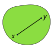
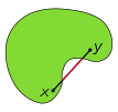
Convexity in economics
| Part of a series on |
| Economics |
|---|
Convexity is an important topic in economics.
Preliminaries
This section may contain material not related to the topic of the article and should be moved to convex analysis instead. (August 2013) ) |
The economics depends upon the following definitions and results from convex geometry.
Real vector spaces
A real vector space of two dimensions may be given a Cartesian coordinate system in which every point is identified by a list of two real numbers, called "coordinates", which are conventionally denoted by x and y. Two points in the Cartesian plane can be added coordinate-wise
- (x1, y1) + (x2, y2) = (x1+x2, y1+y2);
further, a point can be multiplied by each real number λ coordinate-wise
- λ (x, y) = (λx, λy).
More generally, any real vector space of (finite) dimension D can be viewed as the
Convex sets
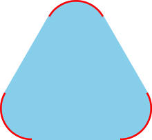
In a real vector space, a set is defined to be is convex.
More formally, a set Q is convex if, for all points v0 and v1 in Q and for every real number λ in the unit interval [0,1], the point
- (1 − λ) v0 + λv1
is a member of Q.
By
The definition of a convex set implies that the intersection of two convex sets is a convex set. More generally, the intersection of a family of convex sets is a convex set.
Convex hull
For every subset Q of a real vector space, its
Duality: Intersecting half-spaces
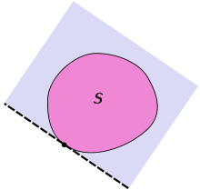
Supporting hyperplane is a concept in geometry. A hyperplane divides a space into two half-spaces. A hyperplane is said to support a set in the real n-space if it meets both of the following:
- is entirely contained in one of the two closed half-spaces determined by the hyperplane
- has at least one point on the hyperplane.
Here, a closed half-space is the half-space that includes the hyperplane.
Supporting hyperplane theorem

This theorem states that if is a closed convex set in and is a point on the boundary of then there exists a supporting hyperplane containing
The hyperplane in the theorem may not be unique, as noticed in the second picture on the right. If the closed set is not convex, the statement of the theorem is not true at all points on the boundary of as illustrated in the third picture on the right.

Economics
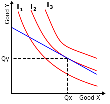
An optimal basket of goods occurs where the consumer's convex preference set is supported by the budget constraint, as shown in the diagram. If the preference set is convex, then the consumer's set of optimal decisions is a convex set, for example, a unique optimal basket (or even a line segment of optimal baskets).
For simplicity, we shall assume that the preferences of a consumer can be described by a
. (The meanings of "closed set" is explained below, in the subsection on optimization applications.)Non-convexity
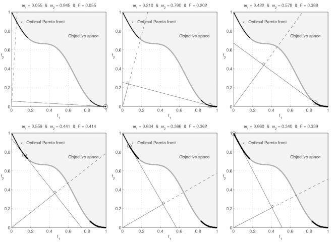
If a preference set is non‑convex, then some prices produce a budget supporting two different optimal consumption decisions. For example, we can imagine that, for zoos, a lion costs as much as an eagle, and further that a zoo's budget suffices for one eagle or one lion. We can suppose also that a zoo-keeper views either animal as equally valuable. In this case, the zoo would purchase either one lion or one eagle. Of course, a contemporary zoo-keeper does not want to purchase a half an eagle and a half a lion (or a griffin)! Thus, the contemporary zoo-keeper's preferences are non‑convex: The zoo-keeper prefers having either animal to having any strictly convex combination of both.
Non‑convex sets have been incorporated in the theories of general economic equilibria,[4] of market failures,[5] and of public economics.[6] These results are described in graduate-level textbooks in microeconomics,[7] general equilibrium theory,[8] game theory,[9] mathematical economics,[10] and applied mathematics (for economists).[11] The Shapley–Folkman lemma results establish that non‑convexities are compatible with approximate equilibria in markets with many consumers; these results also apply to production economies with many small firms.[12]
In "
Nonsmooth analysis
This section may require cleanup to meet Wikipedia's quality standards. The specific problem is: Relationship between subderivatives and non‑convexity remains cryptic. (August 2013) |
Economists have increasingly studied non‑convex sets with nonsmooth analysis, which generalizes convex analysis. "Non‑convexities in [both] production and consumption ... required mathematical tools that went beyond convexity, and further development had to await the invention of non‑smooth calculus" (for example, Francis Clarke's locally Lipschitz calculus), as described by Rockafellar & Wets (1998)[23] and Mordukhovich (2006),[24] according to Khan (2008).[3] Brown (1991, pp. 1967–1968) wrote that the "major methodological innovation in the general equilibrium analysis of firms with pricing rules" was "the introduction of the methods of non‑smooth analysis, as a [synthesis] of global analysis (differential topology) and [of] convex analysis." According to Brown (1991, p. 1966), "Non‑smooth analysis extends the local approximation of manifolds by tangent planes [and extends] the analogous approximation of convex sets by tangent cones to sets" that can be non‑smooth or non‑convex.[25] Economists have also used algebraic topology.[26]
See also
- Convex duality
Notes
- ^ a b c Newman (1987c)
- ^ a b Newman (1987d)
- ^ ISBN 978-0-333-78676-5.
- MR 0389160.
- ISBN 978-0-262-19443-3.
- ISBN 978-0-262-12127-9.
- ISBN 978-0-19-507340-9.
- ISBN 978-0-521-31988-1.
- MR 0700688.
- MR 0657578.
- S2CID 117240618.
- MR 0737006.
- ^ MR 0443878.)
- S2CID 6458099.
- JSTOR 1907054.
- ISBN 978-0-19-506553-4.
- ISBN 978-0-521-31112-0.
- ISBN 9780521348010.
nonconvex OR nonconvexities.
- JSTOR 1909602.
- Drèze, Jacques H.(1974). "Investment under private ownership: Optimality, equilibrium and stability". In Drèze, J. H. (ed.). Allocation under Uncertainty: Equilibrium and Optimality. New York: Wiley. pp. 129–165.)
- ^ Page 371: Magill, Michael; Quinzii, Martine (1996). "6 Production in a finance economy, Section 31 Partnerships". The Theory of incomplete markets. Cambridge, Massachusetts: MIT Press. pp. 329–425.
- ISBN 9780333786765.
- S2CID 198120391.
- MR 2191745.
- MR 1207195.
- MR 1218037.
References
- ISBN 978-0-333-78676-5.
- Blume, Lawrence E. (2008b). "Convex programming". In Durlauf, Steven N.; Blume, Lawrence E (eds.). The New Palgrave Dictionary of Economics (Second ed.). Palgrave Macmillan. pp. 220–225. ISBN 978-0-333-78676-5.
- Blume, Lawrence E. (2008c). "Duality". In Durlauf, Steven N.; Blume, Lawrence E (eds.). The New Palgrave Dictionary of Economics (Second ed.). Palgrave Macmillan. pp. 551–555. ISBN 978-0-333-78676-5.
- Crouzeix, J.-P. (2008). "Quasi-concavity". In Durlauf, Steven N.; Blume, Lawrence E (eds.). The New Palgrave Dictionary of Economics (Second ed.). Palgrave Macmillan. pp. 815–816. ISBN 978-0-333-78676-5.
- Diewert, W. E. (1982). "12 Duality approaches to microeconomic theory". In MR 0648778.
- Green, Jerry; Heller, Walter P. (1981). "1 Mathematical analysis and convexity with applications to economics". In MR 0634800.
- Luenberger, David G. Microeconomic Theory, McGraw-Hill, Inc., New York, 1995.
- ISBN 9780333786765.
- ISBN 9780333786765.
- ISBN 9780333786765.
- MR 0274683..
- Schneider, Rolf (1993). Convex bodies: The Brunn–Minkowski theory. Encyclopedia of mathematics and its applications. Vol. 44. Cambridge: Cambridge University Press. pp. xiv+490. MR 1216521.

