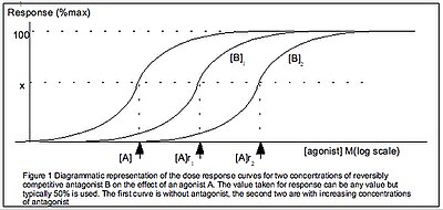
Dose–response relationship
This article needs additional citations for verification. (August 2018) |

The dose–response relationship, or exposure–response relationship, describes the magnitude of the
Motivation for studying dose–response relationships
Studying dose response, and developing dose–response models, is central to determining "safe", "hazardous" and (where relevant) beneficial levels and dosages for drugs, pollutants, foods, and other substances to which humans or other
Example stimuli and responses
Some example measures for dose–response relationships are shown in the tables below. Each sensory stimulus corresponds with a particular
| Example Stimulus | Target | |
|---|---|---|
| Drug/Toxin dose | Agonist (e.g. nicotine, isoprenaline) |
Biochemical receptors, Enzymes, Transporters |
| Antagonist (e.g. ketamine, propranolol) | ||
| Allosteric modulator (e.g. Benzodiazepine) | ||
| Temperature | Temperature receptors
| |
| Sound levels | Hair cells | |
| Illumination/Light intensity | Photoreceptors | |
| Mechanical pressure | Mechanoreceptors | |
| Pathogen dose (e.g. LPS) | n/a | |
| Radiation intensity | n/a | |
| System Level | Example Response |
|---|---|
| Population (Epidemiology) | Death,[4] loss of consciousness |
| Organism/Whole animal (Physiology) | Severity of lesion,[4] blood pressure,[4] heart rate, extent of movement, attentiveness, EEG data |
Organ/Tissue
|
ATP production, proliferation, muscle contraction, bile production, cell death |
| Cell (Cell biology, Biochemistry) | ATP production, calcium signals, morphology, mitosis |
Analysis and creation of dose–response curves

Construction of dose–response curves
doi:10.1007/0-387-33706-7_10 § 10.2. . (April 2023) |
A dose–response curve is a
Statistical analysis of dose–response curves may be performed by regression methods such as the
Typical experimental design for measuring dose-response relationships are organ bath preparations, ligand binding assays, functional assays, and clinical drug trials.
Specific to response to doses of radiation the Health Physics Society (in the United States) has published a documentary series on the origins of the linear no-threshold (LNT) model though the society has not adopted a policy on LNT."
Hill equation
Logarithmic dose–response curves are generally
The Hill equation is the following formula, where is the magnitude of the response, is the drug concentration (or equivalently, stimulus intensity) and is the drug concentration that produces a 50% maximal response and is the
The parameters of the dose response curve reflect measures of potency (such as EC50, IC50, ED50, etc.) and measures of efficacy (such as tissue, cell or population response).
A commonly used dose–response curve is the EC50 curve, the half maximal effective concentration, where the EC50 point is defined as the inflection point of the curve.
Dose response curves are typically fitted to the Hill equation.
The first point along the graph where a response above zero (or above the control response) is reached is usually referred to as a threshold dose. For most beneficial or recreational drugs, the desired effects are found at doses slightly greater than the threshold dose. At higher doses, undesired
The Hill equation can be used to describe dose–response relationships, for example ion channel-open-probability vs. ligand concentration.[9]
Dose is usually in milligrams,
Emax model
The Emax model is a generalization of the Hill equation where an effect can be set for zero dose. Using the same notation as above, we can express the model as:[10]
Compare with a rearrangement of Hill:
The Emax model is the single most common model for describing dose-response relationship in drug development.[10]
Shape of dose-response curve
The shape of dose-response curve typically depends on the topology of the targeted reaction network. While the shape of the curve is often monotonic, in some cases non-monotonic dose response curves can be seen.[11]
Limitations
The concept of linear dose–response relationship, thresholds, and all-or-nothing responses may not apply to non-linear situations. A threshold model or linear no-threshold model may be more appropriate, depending on the circumstances. A recent critique of these models as they apply to endocrine disruptors argues for a substantial revision of testing and toxicological models at low doses because of observed non-monotonicity, i.e. U-shaped dose/response curves.[12]
Dose–response relationships generally depend on the exposure time and exposure route (e.g., inhalation, dietary intake); quantifying the response after a different exposure time or for a different route leads to a different relationship and possibly different conclusions on the effects of the stressor under consideration. This limitation is caused by the complexity of biological systems and the often unknown biological processes operating between the external exposure and the adverse cellular or tissue response.[citation needed]
Schild analysis
This section needs expansion. You can help by adding to it. (April 2019) |
See also
References
- PMID 975067.
- ^ Lockheed Martin (2009). Benchmark Dose Software (BMDS) Version 2.1 User's Manual Version 2.0 (PDF) (Draft ed.). Washington, DC: United States Environmental Protection Agency, Office of Environmental Information.
- ^ "Exposure-Response Relationships — Study Design, Data Analysis, and Regulatory Applications" (PDF). Food and Drug Administration. 26 March 2019.
- ^ PMID 7333256.
- .
- ISBN 9780471816430.
- PMID 26424192.
- S2CID 1729572.
- PMID 10228183.
- ^ ISBN 978-0-387-29074-4.
- PMID 22419778.
External links
- Online Tool for ELISA Analysis
- Online IC50 Calculator
- Ecotoxmodels A website on mathematical models in ecotoxicology, with emphasis on toxicokinetic-toxicodynamic models
- CDD Vault, Example of Dose-Response Curve fitting software


![{\displaystyle {\ce {[A]}}}](https://wikimedia.org/api/rest_v1/media/math/render/svg/881146b6653b24508d87e34a81c84832f1d5ffea)


![{\displaystyle {\frac {E}{E_{\mathrm {max} }}}={\frac {[A]^{n}}{{\text{EC}}_{50}^{n}+[A]^{n}}}={\frac {1}{1+\left({\frac {\mathrm {EC} _{50}}{[A]}}\right)^{n}}}}](https://wikimedia.org/api/rest_v1/media/math/render/svg/2f925d0aa80958bffa0823bb0af1776f883c85e0)
![{\displaystyle E=E_{0}+{\frac {{[A]}^{n}\times {E_{\mathrm {max} }}}{{[A]}^{n}+\mathrm {EC} _{50}^{n}}}}](https://wikimedia.org/api/rest_v1/media/math/render/svg/ba22280d1fc6d1db52bf0ae46800e77d582b632f)
![{\displaystyle E_{\mathrm {hill} }={\frac {{[A]}^{n}\times {E_{\mathrm {max} }}}{{[A]}^{n}+\mathrm {EC} _{50}^{n}}}}](https://wikimedia.org/api/rest_v1/media/math/render/svg/12552d523bba224b4d70fea7e1cbbc2d6781792a)