
User:Epipelagic/sandbox/ref2
| This is a Wikipedia user page. This is not an encyclopedia article or the talk page for an encyclopedia article. If you find this page on any site other than Wikipedia, you are viewing a mirror site. Be aware that the page may be outdated and that the user in whose space this page is located may have no personal affiliation with any site other than Wikipedia. The original page is located at https://en.wikipedia.org/wiki/User:Epipelagic/sandbox/ref2. |
RESOURCES AND WORKING DRAFTS ONLY
Seagrass and sea cucumbers

Tropical seagrass meadows are among the most productive ecosystems in the coastal zones. They have an important role in stabilizing bottom sediments (Den Hartog, 1970), reducing the water current and thereby promoting sedimentation and settlement of planktonic larvae (Agawin and Duarte, 2002; Panyawai et al., 2019; Mercier et al., 2000), providing habitat for resident and transient fauna (Den Hartog, 1979; Heck et al., 2008; Ralph et al., 2013; Nishihama and Tanita, 2021) sustaining high primary production (Estacion and Fortes, 1988; Calumpong and Meñez, 1994; Rattanachot and Prathep, 2011), promoting carbon sequestration from autochthonous and allochthonous sources (Duarte et al., 2004; Kon et al., 2015; Trevathan-Tackett et al., 2017; Stankovic et al., 2021), providing protection from predators as a function of habitat complexity (Orth et al., 1984; Hair et al., 2020), supporting direct grazing (Thayer et al., 1984; Cebrián and Duarte, 1998), and assimilating seagrass particulate organic matter (Ricart et al., 2015; Domínguez-Godino et al., 2019; Floren et al., 2021). In return, seagrasses benefit from the burrowing activities of faunal communities, such as sea cucumbers, resulting in a considerable increase in the growth rates of seagrass leaves (Arnull et al., 2021). Additionally, sea cucumbers play a vital role as bioturbators or ecosystem engineers in the sediments that promote recycling of nutrients within the seagrass meadows (Uthicke and Klumpp, 1998; Costa et al., 2014; Lee, 2016). Despite the ecological and economic functions of seagrass meadows and associated fauna, this ecosystem suffers due to coastal developments and regular typhoons that affect its proper functioning.[1]
Perhaps one of the most valuable faunas associated with the tropical seagrass meadows is the sea cucumber. The Holothuridae and Stichopodidae families form an important part of the fishery industry that has been in existence in the Indo-Pacific for over 1000 years (Bruckner et al., 2003). This association of sea cucumbers with the seagrasses received considerable attention in recent times due to the intense fishing pressure on this vital resource in the wild (e.g., Mercier et al., 2000; Hamel et al., 2001; Domínguez-Godino et al., 2019), prompting authorities to seek for solutions aimed at restoring depleted stocks. Despite the restoration initiatives being undertaken to mitigate the depleting sea cucumber populations, managing the wild sea cucumber fisheries has been proven largely unsuccessful (e.g., Choo, 2008; Vincent and Morrison-Saunders, 2013; Robinson and Lovatelli, 2015). One of the causes for this failure is the general lack of understanding of the underlying mechanisms that characterize this trophic relationship.[1]
- ^ ISSN 2296-7745..
{{cite journal}}: CS1 maint: unflagged free DOI (link) Modified material was copied from this source, which is available under a Creative Commons Attribution 4.0 International License
Research history (biogeochemical cycles)


Ancient foreshadowing
Perhaps the earliest examples of conceptually linking organic and inorganic substances with large earth cycles (the rudiments of biogeochemical cycles) can be traced to Empedocles (483–424 B.C.) who divided the physical universe into air, water, fire, and earth, as well as to a disciple of Confucius (551–479 B.C.) who developed a five universal element system.[2][3][4]
The
- Lai, K. L. (2003). Classical China. In: D. Jamieson (Ed.), A Companion to Environmental Philosophy (pp. 21-36). Oxford: Blackwell.
Zou Yan established a school which promoted his teachings, the
His theory attempted to explain the universe in terms of basic forces in nature: the complementary agents of yin (dark, cold, female, negative) and yang (light, hot, male, positive) and the Five Elements or Five Phases (water, fire, wood, metal, and earth).
Age of enlightenment
However, as the Canadian biogeochemist
"The concept played little part in scientific thought, however, until the publication, first in Russian in 1926 (actually 1924) and later in French in 1929 (under the title La Biosphere), of two lectures by the Russian mineralogist
Jean Baptiste Lamarck, whose geochemistry, although archaically expressed, was often quite penetrating".
The boundaries between these different physical states of rock, gas, water, and organic matter (Fig. 1) change when phase transitions are thermodynamically in favor of a molecule that is catalyzed into transition to another state; understanding the controls of these transitions in the biosphere is central to biogeochemistry.[4][1]
In 1795, the Scottish geologist
The French chemist
Quite remarkably, much was learned during this time period about the linkages between
Finally, it should also be noted here, that the importance of the
Microbial worlds
While the chemistry of agriculture continued to develop there remained a lack of understanding of how microbes specifically interfaced with key elemental cycles. We now see
In a microbial world
In the 19th century, the importance of bacteria proved to be an important step understanding nitrification in soils (e.g. Winogradsky 1891)—this combination of lab and field techniques proved to be pivotal in the history of microbial ecology and biogeochemistry. In 1913, Beijerinck was the first to use the term micooekologie, or as we think of it today,
As noted in the Falkowski et al. (2008) paper entitled The Microbial Engines That Drive Earth’s Biogeochemical Cycles': Earth is ~ 4.5 billion years old, and during the first half of its evolutionary history, a set of metabolic processes that evolved exclusive in microbes would come to alter the chemical speciation of virtually all elements on the planetary surface. Consequently, our current environment reflects the historically integrated outcomes of microbial experimentation on a tectonically active planet endowed with a thin film of liquid water."[1]
The importance of microbes as transformers of energy in the ocean really began to take shape in the 1970s and 1980s, which set the stage of future
- ^ ISSN 0168-2563.. Modified text was copied from this source, which is available under a Creative Commons Attribution 4.0 International License
- ^ A Source Book of Agricultural Chemistry, By Charles A. Browne. 1944. Retrieved 12 July 2022.
- ISBN 978-0-415-32505-9. Retrieved 2022-07-13.
- ^ ISBN 978-3-642-48879-5. Retrieved 2022-07-13.
- ^ Russell (1991), p. 72.
- ^ Russell (1991), p. 61.
- ^ Russell (1991), p. 46.
- ^ Curd (2020).
- ^ Russell (1991), pp. 62, 75.
- ISBN 0-521-21821-7
- doi:10.1007/BF00002942.)
{{cite journal}}: Cite journal requires|journal=(help); Missing or empty|title=(help
Plant–animal interactions
![Plant–animal interaction such as pollination, herbivory, frugivory, and mutualism. Biological signatures in the form of eDNA or eRNA can be detected from plants noninvasively to trace out complex interactions.[1]](/File:Plant%E2%80%93animal_interaction_and_eDNA.jpg)
One of the principal means by which taxa are interconnected in nature is via plant–animal interactions (PAI). These interactions can play pivotal ecological roles and materialize in multiple combinations of positive and antagonistic relationships (e.g., predation, frugivory and herbivory, parasitism, and mutualism). For example, frugivory contributes to propagation and thus facilitates plant restoration [2][3] and gene flow.[4] Without such mutualistic relationships, some plants may not be able to complete their life cycles, and the animals may starve due to resource deficiency. Herbivory leads to defoliation or root removal, which can regulate or diminish overall phytomass but can also increase species diversity and influence plant distribution,[5][6] thereby regulating ecosystem stability.[5] [7][8] In pollinator-plant mutualisms, the former acquires feeding from the latter and in return serves as an agent of plant propagation and a vector for gene flow.[9] Studies documenting the food habits of pollinators and their interactive role in sustaining ecosystems have already shed light on the complex network of species-specificity, habitat preference, and coevolution between plants and their pollinators.[10] Mutualisms also assist with growth and offer protection from pathogens (e.g., plant–insect associations.[11] In contrast, antagonistic interactions (e.g., parasites and parasitoids) can affect the growth of plants and result in economical and ecological loss.[12] Thus, PAI underpins many of the fundamental processes related to ecosystem structure and functioning.[13][1]
However, studying these multifaceted interactions using conventional methods (e.g., field observation, camera, malaise, pitfall traps, and gut content analysis) is often difficult and laborious[14] Alternatively, molecular advancements with the analysis of trace DNA from environmental samples (i.e., environmental DNA or “eDNA”) have provided researchers and managers the ability to scale up documentation and monitoring of such relationships, and to do so at increased spatiotemporal frequencies with more cost-effectiveness.[1]
Methodological development for the application of eDNA has rapidly evolved from the presence/absence detection of organisms (Ficetola et al., 2008) and abundance quantification of eDNA signals (Taberlet et al., 2012), to the detection of whole communities (Deiner et al., 2021) and even their trophic interactions (D'Alessandro & Mariani, 2021; Thomsen & Sigsgaard, 2019). Indeed, eDNA-based methods have experienced a sharp adoption in different fields such as conservation biology (e.g., detection of endangered or invasive species; Piaggio et al., 2014; Stewart et al., 2017), ecological biomonitoring in the terrestrial and aquatic ecosystem (e.g., environmental health monitoring; Xie et al., 2017), wildlife forensics (Allwood et al., 2020), wildlife disease monitoring (Barnes et al., 2020), and animal behavior (Nichols et al., 2015). The application of eDNA methods to investigate a myriad of ecological interactions such as pollination (e.g., plant-insects, plant–animal), predation (e.g., herbivory, frugivory), and mutualism (e.g., plant–nematode, plant–insect, plant–animals) (Rasmussen et al., 2021; Thomsen & Sigsgaard, 2019; van Beeck Calkoen et al., 2019) further demonstrates the application of eDNA as a multidisciplinary approach (Deiner et al., 2021; Veilleux et al., 2021) poised to tackle complex ecological questions regarding inter-taxa relationships.[1]
Loss of species interactions may occur well before the actual extinction of individual species, thereby initiating deleterious effects on species functionality and its service to the ecosystem.[15] This in turn further accelerates species extinction rates (Simmons et al., 2020), which is especially pertinent for specialist species (Colles et al., 2009). In fact, given that the loss of successive interactions provides an early warning system for the deterioration of ecosystem health (Valiente-Banuet et al., 2015), documenting, monitoring, and conserving such complex interactions is critical to retain ecosystem functioning.[1]
- ^ ISSN 2637-4943.. Modified text was copied from this source, which is available under a Creative Commons Attribution 4.0 International License
- doi:10.1371/journal.pone.0054956.)
{{cite journal}}: Cite journal requires|journal=(help); Missing or empty|title=(help)CS1 maint: unflagged free DOI (link - doi:10.1007/s12686-018-1074-4.)
{{cite journal}}: Cite journal requires|journal=(help); Missing or empty|title=(help - doi:10.1111/j.1365-294X.2007.03427.x.)
{{cite journal}}: Cite journal requires|journal=(help); Missing or empty|title=(help - ^ doi:10.1002/ece3.2950.)
{{cite journal}}: Cite journal requires|journal=(help); Missing or empty|title=(help - doi:10.2307/2937150.)
{{cite journal}}: Cite journal requires|journal=(help); Missing or empty|title=(help - doi:10.1890/11-2067.1.)
{{cite journal}}: Cite journal requires|journal=(help); Missing or empty|title=(help - doi:10.1002/ece3.1647.)
{{cite journal}}: Cite journal requires|journal=(help); Missing or empty|title=(help - doi:10.1093/beheco/ars019.)
{{cite journal}}: Cite journal requires|journal=(help); Missing or empty|title=(help - doi:10.1016/j.tree.2007.11.003.)
{{cite journal}}: Cite journal requires|journal=(help); Missing or empty|title=(help - doi:10.1002/edn3.131.)
{{cite journal}}: Cite journal requires|journal=(help); Missing or empty|title=(help - doi:10.1371/journal.pone.0117872.)
{{cite journal}}: Cite journal requires|journal=(help); Missing or empty|title=(help)CS1 maint: unflagged free DOI (link - doi:10.1007/s12210-008-0005-9.)
{{cite journal}}: Cite journal requires|journal=(help); Missing or empty|title=(help - doi:10.1002/ece3.4809.)
{{cite journal}}: Cite journal requires|journal=(help); Missing or empty|title=(help - doi:10.1111/1365-2435.12356.)
{{cite journal}}: Cite journal requires|journal=(help); Missing or empty|title=(help
microbial ecology
- The evolution of microbial ecology of the ocean <<<<< —————— <<<<<
- Scientists’ warning to humanity: microorganisms and climate change
- Microbial ecology‐based engineering of Microbial Electrochemical Technologies
holobiont asides
Seaweed holobiont
Marine

Several studies have already highlighted the importance of interkingdom interactions, which can be essential for the physiology of all partners (Wichard et al., 2015). In that respect, some bacterial strains have been shown to be involved in the
Abalone holobiont

Plant microbiome
- create article - this includes copy from microbiome, microbiota, root microbiome, Evolutionary history of plants and holobiont – see those page's histories for attribution

The plant microbiome encompasses a community of distinct microbial groups, such as prokaryotes (bacteria and archaea), fungi, protists (algae and protozoa) and viruses.
"Plant genomes contribute to the structure and function of the plant microbiome, a key determinant of plant health and productivity. High-throughput technologies are revealing interactions between these complex communities and their hosts in unprecedented detail."[6]
"The plant microbiome is a key determinant of plant health and productivity,[7] and has received substantial attention in recent years.[8][9] A testament to the importance of plant-microbe interactions are the mycorrhizal fungi. Molecular evidence suggests that their associations with green algae were fundamental to the evolution of land plants about 700 million years ago.[10] Most plants, although notably not Arabidopsis thaliana and other Brassicaceae, have maintained this symbiosis, which assists root uptake of mineral nutrients such as phosphate.[11] Plant-associated microbes are also key players in global biogeochemical cycles.[12] A significant amount, 5 to 20%, of the products of photosynthesis (the photosynthate) is released, mainly into the rhizosphere (the soil-root interface) through roots.[13] In addition, 100 Tg of methanol and 500 Tg of isoprene are released into the atmosphere by plants annually.[14][15] For methanol this corresponds to between 0.016% and 0.14% of photosynthate depending on plant type.[14] Both are potential sources of carbon and energy for microorganisms. In agricultural soils in particular, plants stimulate microbial denitrification and methanogenesis, which contribute to emissions of N2O and methane, respectively.[16][17] These gases represent a loss of carbon and nitrogen from the system and contribute to the greenhouse effect."[6]
Sidebar
| Part of a series on |
Microbiomes |
|---|
 |
Plant microbiota
- Microbial structures
- The
"Healthy plants host diverse but taxonomically structured communities of microorganisms, the


In the diagram on the right, microbiota colonizing the rhizosphere, entering the roots and colonizing the next tuber generation via the stolons, are visualized with a red color. Bacteria present in the mother tuber, passing through the stolons and migrating into the plant as well as into the next generation of tubers are shown in blue.[22]
- The soil is the main reservoir for bacteria that colonize potato tubers
- Bacteria are recruited from the soil more or less independent of the potato variety
- Bacteria might colonize the tubers predominantly from the inside of plants via the stolon
- The bacterial microbiota of potato tubers consists of bacteria transmitted from one tuber generation to the next and bacteria recruited from the soil colonize potato plants via the root.[22]
Plants are attractive hosts for microorganisms since they provide a variety of nutrients. Microorganisms on plants can be
- Cited by 939: Vorholt, J.A., 2012. Microbial life in the phyllosphere. Nature Reviews Microbiology, 10(12), pp.828-840.
- Cited by 616: Turner, T.R., James, E.K. and Poole, P.S., 2013. The plant microbiome. Genome biology, 14(6), pp.1-10.
The plant "theatre of activity"
The plant "theatre of activity" "includes microbial structures,
Overview
"In the past decade, a paradigm shift in the life sciences has emerged in which microbial communities are viewed as functional drivers of their eukaryotic hosts. For plants, microbiomes can expand the genomic and metabolic capabilities of their hosts, providing or facilitating a range of essential life-support functions, including nutrient acquisition, immune modulation, and (a)biotic stress tolerance. While plant microbiomes have been proposed as a new platform for the next green revolution, fundamental knowledge of the mechanisms underlying microbiome assembly and activity is still in its infancy. Plant microbiologists have started to embrace the full breadth of high-throughput sequencing technologies to decipher the intricacies of the functional diversity and spatiotemporal dynamics of plant microbiomes. Our ability to go beyond one-microbe-at-atime approaches has already led to a more holistic view of the plant microbiome and the discovery of taxonomically novel microorganisms and beneficial microbial consortia (27, 51, 91). Also, de novo assembly of microbial genomes from metagenome data has been leading to the identification of novel genes and pathways involved in microbe-microbe and microbe-plant interactions (4, 20, 27, 50, 65, 74, 84).[30]
Microbiome research has also attracted the attention of various other research disciplines, including botany and plant ecology (42, 87, 100, 144), restoration and invasion ecology (64, 142), phytoremediation (119), mathematics and modelling (59, 92), and chemistry and natural product discovery (36). The striking similarities with the human microbiome (12, 43, 85) have further fueled the conceptual framework of plant microbiome research and stimulated the development of microbiome-based strategies to improve plant growth and health (34, 114, 129). For example, the colonization potential of an introduced microbial species (probiotic) is a fundamental aspect of human microbiome research and health care, but it is also a key element of the successful implementation of microbial inoculants for plant growth promotion and disease control (15). The overall results obtained so far indicate that introduced microorganisms are usually washed out and do not persist in the gut, plant, or soil ecosystem at functionally meaningful densities (39, 79, 114, 138). In this context, it is of fundamental importance to understand the coevolutionary trajectories of plant microbiomes and the mechanisms underlying assembly, activity, and persistence. 7"[30]
"The causes and consequences of plant-associated microbial variation have been the subject of intense study for over a century. Following the discovery that atmospheric nitrogen is fixed by bacteria residing in leguminous root nodules came the understanding that plants are associated with an abundance of diverse microbes. Hypotheses that arose in that period are fundamental to the field to this day. Among them are the notions articulated by Lorenz Hiltner (60): that plant-derived nutrients attract beneficial microbiota in a species-specific manner and that this mechanism is exposed to exploitation by pathogens. For over a century, the field relied on culture-dependent approaches to illuminate and study the multitude of plant microbiome inhabitants, which include fungi, bacteria, protists, and viruses. However, the stunning extent and distribution of this diversity revealed by culture-independent and high-throughput molecular approaches over the past two decades have had a transformative effect on our understanding, study, and application of plant-microbe research."[31]
Cited by 205...
"The plant microbiome has been considered one of the key determinants of plant health and productivity for over 100 years, and intensive research on this topic started with Lorenz Hiltner's work in 1901 (Hartmann et al., 2008). This long research period was influenced by the continuous development of research methods, but it was the application of molecular and omics techniques, as well as novel microscopic techniques combining molecular and analytical tools, that led to the important milestones (Muyzer and Smalla, 1998; Caporaso et al., 2012; Jansson et al., 2012). For example, deeper insights into the structure and function of plant-associated microbial communities of the model plant Arabidopsis were presented by Bulgarelli et al. (2012) and Lundberg et al. (2012), while another study detailed a disease-suppressive rhizosphere microbiome in sugar beet (Mendes et al., 2011). The last century has been characterized by important, diverse, and unexpected discoveries relating to plant-associated microorganisms that were made by applying several research methods, especially combinations thereof. Several selected examples are as follows: (i) the potential of root-associated microbes to suppress soil-borne pathogens, demonstrated by strain selection and field trials (Cook et al., 1995; Weller et al., 2002); (ii) trans-kingdom communication between plants and microbes, analysed by analytical and molecular methods (Hartmann and Schikora, 2012); (iii) plant species-specific rhizosphere microbial communities, obtained by molecular fingerprints and molecular strain analysis (Berg and Smalla, 2009; Hartmann et al., 2009); (iv) the rhizosphere as a reservoir of facultative human pathogens, detected by isolation and characterization of strains (Berg et al., 2005), and deep study of the lettuce metagenome (Berg et al., 2014a); (v) the high diversity and importance of the endophytic (myco)biome visualized especially by fluorescence in situ hybridization and microscopy (Omacini et al., 2001; Rodriguez et al., 2009; Hardoim et al., 2015); and (vi) the detection of abundant endophytic Archaea in trees using molecular markers based on genomics of non-cultivable organisms (Müller et al., 2015)."[32]
"From protists to humans, all organisms are inhabited by microorganisms. According to the holobiont concept, metaorganisms are co-evolved species assemblages. Moreover, co-evolution has resulted in intimate relationships forming between microbes and their hosts that create specific and stable microbiomes. Therefore, all eukaryotic organisms can be considered to be metaorganisms: an association of the macroscopic hosts and a diverse microbiome consisting of bacteria, archaea, fungi, and protists (even protists can have their own bacterial microbiota, and it has been argued that microbiota play an important role in the evolution of multicellularity; McFall-Ngai et al., 2013). Together, microbiota fulfil all important functions for the holobiont themselves, and also for the ecosystem (Mendes and Raaijmakers, 2015; Vandenkoornhuyse et al., 2015). Interestingly, in addition to the joint fulfilment of tasks, many organisms have ‘outsourced’ some essential functions, including those of their own development, to symbiotic organisms living with them (Gilbert et al., 2012)."[32]
"Plants harbour different microbial communities specific for each plant organ, for example the phyllosphere (Vorholt, 2012), rhizosphere (Berendsen et al., 2012; Philippot et al., 2013), and endosphere (Hardoim et al., 2015). The rhizosphere is the most studied habitat owing to its enormous potential for plant nutrition and health (Berendsen et al., 2012; Hirsch and Mauchline, 2012; Bakker et al., 2013; Mendes et al., 2013). It has been known for many years that the rhizosphere enriches specific microbial species/genotypes in comparison to soil and inner tissues, but modern technologies provide much deeper insights and expand our understanding of plant–microbe interactions (Bais et al., 2006; Doornbos et al., 2012). A current model shows the occurrence of seed-borne microorganisms (Christin Zachow and Gabriele Berg, personal communication) and the attraction of microbes to nutrients such as carbohydrates and amino acids (Moe, 2013) in combination with plant-specific secondary metabolites (Weston and Mathesius, 2013). Plant root exudates play important roles as both chemo-attractants and repellents (Badri and Vivanco, 2009). Additionally, plant defence signalling plays a role in this process (Doornbos et al., 2012). The importance of the rhizosphere microbiome can be underlined by the number of species: in the metagenomes studied in our group, we found up to 1200 prokaryotic species (extracted 16S rRNA genes annotated using the Greengenes reference database). Moreover, a higher number of species was found in medicinal and wild plants than on crops grown in intensive agriculture (Martina Köberl and Gabriele Berg, personal communication). For comparative analyses, all metagenomes were rarefied at a sequencing depth of 1.7×10⁷ sequences; the actual species diversity is even much higher. The abundances measured sum up to 109–1011 bacterial cells colonizing each gram of the root, which often not only outnumbers the cells of the host plants but also represent more microbes than people existing on Earth. While the well-studied rhizosphere represents the soil–plant interface, the phyllosphere forms the air–plant interface. This microhabitat is also of special interest owing to its large and exposed surface area and its connection to the air microbiome, especially air-borne pathogens (Vorholt, 2012). In our metagenomes, we found a lower microbial diversity in the phyllosphere than in the rhizosphere, but the overall diversity was quite large and comprised up to 900 species (Armin Erlacher and Gabriele Berg, personal communication). In general, leaves have different strategies to trigger microbial colonization, for example (antimicrobial) wax layers, (antimicrobial) secondary metabolites, trichomes, and hairs, and the microbial composition seems to be highly individual but also plant-dependent. However, an overview of a broader range of plant phyla is still missing. Recently, the majority of the research has been focused on the endosphere of plants. Although endophytes were defined by De Bary in 1866 as ‘any organisms occurring within plant tissues’, their existence was ignored until the end of the last century, and very often these organisms were considered contaminants. Now, the organisms inhabiting the endosphere are well-accepted and, moreover, their intimate interaction with the plant makes them the focus of (biotechnological) interest. Seeds also harbour a surprisingly diverse microbiome in their endosphere (Johnston-Monje and Raizada, 2011). There are many more micro-environments described, for example the endorhiza (root), the anthosphere (flower), the spermosphere (seeds), and the carposphere (fruit), but their specific microbiome is less studied."[32]

The diagram on the right →
illustrates microbial communities in the soil, air, rhizosphere, phyllosphere, and inside plant tissue (endosphere). In each of these habitats, microbes (represented by colored circles) could interact positively, negatively, or do not interact with other microbes (no lines). Specific microbes, often defined as “hub” or “keystone” species (circles highlighted in bold), are highly connected to other microbes within the networks and likely exert a stronger influence on the structure of microbial communities. (a) Root-associated microbes mainly derive from the soil biome. (b) Leaf-associated microbes originate from various sources such as aerosols, insects, or dust. (c) Relocation between aboveground and belowground microbiota members.[33]
The microbial component of healthy seeds – the seed microbiome – appears to be inherited between plant generations and can dynamically influence germination, plant performance, and survival. As such, methods to optimize the seed microbiomes of major crops could have far-reaching implications for plant breeding and crop improvement to enhance agricultural food, feed, and fiber production.[34]

In the diagram on the right, microbiota colonizing the rhizosphere, entering the roots and colonizing the next tuber generation via the stolons, are visualized with a red color. Bacteria present in the mother tuber, passing through the stolons and migrating into the plant as well as into the next generation of tubers are shown in blue.[22]
- The soil is the main reservoir for bacteria that colonize potato tubers
- Bacteria are recruited from the soil more or less independent of the potato variety
- Bacteria might colonize the tubers predominantly from the inside of plants via the stolon
- The bacterial microbiota of potato tubers consists of bacteria transmitted from one tuber generation to the next and bacteria recruited from the soil colonize potato plants via the root.[22]


(B) Upon infection by a pathogen (red microbe), the exudation profile of roots changes and stress-induced exudates (blue arrows) aid the plants in inhibiting pathogenic growth in the rhizosphere, while selecting at the same time for beneficial microbes. Some of these beneficial microbes when they establish themselves in the rhizosphere, can trigger ISR that can help plants deal with pathogenic infections in the leaves.
(C) In the case of soil suppressiveness or “cry-for-help” conditions, there is establishment of beneficial rhizosphere communities that are further supported by the release of stress-induced exudates. Under these conditions, soilborne and foliar pathogens fail to cause disease.
(D) Plants experiencing nutrient deficiencies (e.g. iron, nitrogen, phosphate) change the metabolomic profile of their roots to either make nutrients more available and soluble or to attract beneficial microbes (e.g. rhizobia, AMF, PGPR) that can help them deal with the nutrient deficiency. Font size indicates the abundance of beneficial or pathogenic subsets of the microbiota under different conditions.[38]

The sessile nature of plants limits their capacity to deal with an immediate and localized disturbance, irrespective of whether the disturbance is caused by biotic or abiotic stress. It therefore stands to reason that plants have evolved systems to manage the impact of these collective and respective stresses. From a biotic microbial view point, plants play host to a number of organisms that reside in the phyllosphere, endosphere, and rhizosphere, influencing how a plant reacts to its environment. If viewed in the context of an ecological unit, the community of organisms is known as the holobiont. Further incorporating the environment results in what is collectively known as the phytobiome, where the possible plant-microbe-stress interactions are shown in the diagram at the right.[39]

The holobiont has a much greater evolutionary potential for dealing with biotic and abiotic stress than the plant itself. Therefore, it is potentially more sustainable to manage abiotic/biotic stresses in a holistic and multifaceted manner. The plant employs a combinatorially complex system of receptors and signals to adapt to different stressors.[40] Unraveling the complexity of the system is not a trivial task, with researchers providing different perspectives for elucidating a contextual understanding of the dynamics of plant-microbiome interaction.[39]
The improved understanding of the interactions between the plant and its microbiome has broadened our knowledge on the capabilities of the plant to influence its microbiome and vice versa. In interacting with its microbiome, plants have the capacity to release chemical signals into their environment. The signals can either have a positive or negative effect on other plants or members of the microbiome. Root exudates, comprised of allelochemicals, have been associated with signaling in plant-microbe interaction and can also facilitate plant to plant communication (Bais et al., 2004). Exudates with potential allelopathic properties can help the plant both positively and negatively select for members of their phytobiome (Bertin et al., 2003; Sasse et al., 2018), allowing the plant to establish a rhizosphere and soil microbiome that may also be beneficial or detrimental to other plants and microbes. The concept of influencing the plant phytobiome has also been explored in biocontrol strategies, e.g., strategies against nematodes (Stirling, 2017). The ability of the plant, together with individual members of its microbiome, to control and shape the overall microbiome influences a plant's growth and stress response. A better understanding of the resultant interplay between defense and control may allow for an optimized holobiont that can benefit, among others, agricultural and bioremediation efforts (Ojuederie and Babalola, 2017; Pappas et al., 2017; Ab Rahman et al., 2018).[39]
Phyllosphere microbiomes
ABSTRACT: "The phyllosphere is one of the largest ecological niches on our planet. It is formed by the plant cuticle, which is a highly impermeable, hydrophobic biopolymer covering all primary aboveground plant organs protecting them against desiccation. Although living conditions in the phyllosphere are considered harsh, a great variety of microorganisms can live within this habitat. Commensals as well as pathogenic can be found on the plant surface competing for niches and rare nutrient sources."[41]
"In the past the main focus of research in plant microbe interaction was dealing with the hidden half of plants, the so-called rhimsphere where uptake and allocation of water as well as minerals by the plant root system take place[42][43] A tremendous amount of plant/microbe interactions is taking place in the rhizosphere.[44][45] In recent years microbiology of the phyllosphere gained increasing significance, and it is no longer neglected. To describe and understand the underlying mechanisms in water and solute transport within the phyllosphere and the entanglement of plant and microbe physiology. combining classical plant ecophysiology with microbiological approaches represent the main research questions in this field."[41]
"The phyllosphere-aerial plant surface, is the largest biological interface on planet Earth, which provides key life sustaining global services such as carbon dioxide fixation, molecular oxygen release, and primary biomass production (Delmotte eI al. 2009) The area of the world's leaf surface habitat is around one billion km2and harbors-10 bacteria (Lindow and Brandt 2003). [Compare with interface to the ocean, which is about 360 million square kilometers] The carrying capacity of phyllosphere to support microbes depends on different carbon and energy sources that are produced by the plant leaves as exudates and metabolites (Lindow and Brandt 2003; Delmotte et al. 2009; Knief at al. 2010; Remus.Emsennann at al 20124 Phyllosphere microbes It as individual cells m aggregations on leaves (Monier and Lindow 2004). Mostly, phyllosphere rematch has fmused on plant pathogens and mechanisms involving pathogenicity such as spread, colonization, succemion, and survival (e.g., Lindow and Brandi 2003) while paying less atten-tion to phyllosphere microbiome diversity and its functions. There are same stud-ies on community composition of the phyllosphere microbiome (Yang et al. 2001; Lambais et al 2006) and describe physiological and adaplational insights of few genera on leaf surfaces (Delmotte at al 2009). Phyllosphcre microbiome performs a number of ecological services, such as N-fixelion, contaminant biodegradation, and pathogen suppression (Lindow and Brandt 2001; Sandhu et al 2007; Fumkrana et at 2008). Fumkranz et al. (2008) suggested that phyllosphere bacteria provide a significant nitrogen input into some rainforest ecosystems. However, phyllosphere bacteria are also recognized as possible pathogens of plants and animals in these system4(Lindow and IBrandt 2003; Lambais et al. 2006) "[46]
Endosphere microbiomes

(inside plant tissue)
- "Defining the root endosphere and rhizosphere microbiomes from the World Olive Germplasm Collection" - .
"The endosphere, which comprises all inner root tissues is and composition of microbial communities are very different between the rhizosphere and the endosphere. These obserations indicate that Me endosphere of plows has the potential to attract EN, Naylor er I, Microbial communities inhabiting the root endosphere also engage in symbiosis, which is defined as bological organisms with Melt host Endophytic communities of the root system aredistinct asserrA. and not mere subsets°, the microbial communities in the rhimsphere (,otta et A., 20111. by sonication Arabidopsis 11,1g.1,11, 201, I undh, et al...21. Recent experiments have on that the host gen,e have relatively Jae effects on the composition et al.. 201x. Lundberg et at., 2,4 A study in rice has (Yu et al., 21114 Moreover, some earliex studia have shown Mat metabolic and genetic fingeminning Jong the root are highly diversified for different plam species (Yang and microbial signatures along the different ma zones (Kawa..ald A., 2014 These discover. demonstrate that distinct out by studying the microbial community structure in whole root system (Kawasak, et al.. 2014 Therefore, it will be necessary to compare root type-specific microbial provIde an evolutionary perspective to the undemanding of how developmental characteristics affect the microbiome in Me endosphere and Mixosphere".[48]

"Since plants cannot move, they face more challenges in acquiring sufficient nutrients from a given site, defending against herbivores and pathogens, and tolerating abiotic stresses including drought, salinity, and pollutants. The plant microbiome may help plants overcome these challenges. Since genetic adaptation is relatively slow in plants, there is a distinct advantage to acquiring an effective microbiome able to more rapidly adapt to a changing environment. Although rhizospheric microorganisms have been extensively studied for decades, the more intimate associations of plants with endophytes, the microorganisms living fully within plants, have been only recently studied. It is now clear, though, that the plant microbiome can have profound impacts on plant growth and health. Comprising an ecosystem within plants, endophytes are involved in nutrient acquisition and cycling, interacting with each other in complex ways. The specific members of the microbiome can vary depending on the environment, plant genotype, and abiotic or biotic stresses.[49][50][51][52][53] The microbiome is so integral to plant survival that the microorganisms within plants can explain as much or more of the phenotypic variation as the plant genotype.[54] In plant biology research, an individual plant should thus be viewed as a whole, the plant along with intimately associated microbiota (a “holobiont”), with the microbiome playing a fundamental role in the adaptation of the plant to environmental challenges".[55][56][57][58]

Rhizosphere microbiomes

- Overview
The rhizosphere is the plant's external gut — George Monbiot, Regenisis
Interactions between plants and diverse microorganisms colonizing their rhizosphere play a central role in determining nature of the relationship. The plant host fitness as well as the microorganisms are influenced by the outcome of such interactions. Environmental and ecological factors leading to perturbations or disruption of this balanced relationship have also a significant impact. The plant rhizosphere is a complex ecosystem serving as a niche for diverse microorganisms (bacteria, archaea, fungi), nematodes and other organisms. Within the rhizosphere the root exudates have a dual function, influencing nutrient availability and organisms in the vicinity of the root, on one hand. On the other, many microorganisms produce phytohormones that alter the root architecture or other compounds, which affect nutrient availability and thereby the competition between neighboring plants. Sometimes their presence can be beneficial for their host plant since they suppress the growth of phytopathogenic microorganisms. Some other rhizosphere microorganisms such as rhizobacteria and some fungi promote directly plant growth or stimulate the plant immune system. All these phenomena have potential practical applications in agriculture.[60]
- Widely cited
Cited by 2153...
"The diversity of microbes associated with plant roots is enormous, in the order of tens of thousands of species. This complex plant-associated microbial community, also referred to as the second genome of the plant, is crucial for plant health. Recent advances in plant–microbe interactions research revealed that plants are able to shape their rhizosphere microbiome, as evidenced by the fact that different plant species host specific microbial communities when grown on the same soil."[61]
"Pathogens can have a severe impact on plant health. The interactions between plants and pathogens are regularly simplified as trench warfare between the two parties, ignoring the importance of additional parties that can significantly affect the infection process. Plants live in close association with the microbes that inhabit the soil in which plants grow. Soil microbial communities represent the greatest reservoir of biological diversity known in the world so far.[62][63][64][65] The rhizosphere, which is the narrow zone of soil that is influenced by root secretions, can contain up to 1011 microbial cells per gram root,[66] and more than 30,000 prokaryotic species.[67] The collective genome of this microbial community is much larger than that of the plant and is also referred to as the plant’s second genome."[61]
"The rhizosphere is the portion of soil that experiences a duvet pressure of plant roots, and is a major sick of root exudates (Fig 4 1) Rhisosphcre is complex eco-system comprising of different microbial loop players such as viruses, bactena, prottsts, mycorrhvac, and other animals. The rhisosphere microbes exhibits a diverse set of metabolic achymes, and are known to buffer anthropogerm (Arshad et al 2007, 2000; Hussain el al 2007, 2009a, 20094, 2009, Saloom et al 20(7, 2000, 2012, 2013, 2015, Saleem 2012) and environmental changes (Saleem and Moe 2014) Plant diversity. community compositton. carbon fixation mechanisms (C4 vs. C3), genotypes, growth .ages, root architectures. litter deposition, exudates chemistry, resources diversity, metabolism biochemical signaling molecules and complex bustrophie interactions determine the size, selection, community simian-ty, structure and function of microblome communities (Phillips et al 2003.Garbeya et al m 21014, Ever and III 2003, Bats et aL 200(4. Lamb et al 2011; Schulz et al 2012)"[68]

- Inoculating plants with microorganisms
"Inoculating medicinal and aromatic plants with nurturing rhizospheric microorganisms enhances plant growth, development, and secondary metabolite production through increased nutrient and moisture availability, repressed pathogens, improved stress tolerance, and increased phytochemical synthesis. The use of growth promoting bacteria and mycorrhizal fungi reduces the need for chemical fertilizers and pesticides applied to cultivated medicinal and aromatic plant species. Only a limited number of commercial rhizospheric microorganisms are currently marketed for medicinal and aromatic plants. As more growers become aware of the beneficial effects of rhizospheric microorganisms, increased demand for microorganism products can be expected.".[70]


Soil microbiomes

...


A cross section of a field is shown with different soil moisture levels. On the right side, plant growth is constrained due to low soil moisture levels. An example of a measurable phenotype is shown (CO2, corresponding to soil respiration), which is the result of combined metabolic interactions between soil microbes and plants. Call out circles correspond to a microscale view of soil consortia residing in spatially discrete soil aggregates. Connectivity between consortia is determined by the extent of the pore volume that is water filled and available for diffusion of chemical signals and metabolites. Bacterial (purple symbols) interactions within consortia are designated with white arrows. Fungal hyphae (green filaments) may bridge spatially discrete consortia. Soil viruses (orange symbols) also play a yet undefined role in regulating the soil metaphenome. Lower panel illustrates different types of models applicable to defining the soil metaphenome; from left to right: biochemical reaction networks squares correspond to bacterial (purple) or fungal (green) metabolites, interspecies interaction networks, and interkingdom interactions.[78][81][82]
The drilosphere


There are five 'arenas' of particular high biological activity in soils: the porosphere, the drilosphere, the rhizosphere, the detritusphere, and the aggregatusphere, Beare et al 1995, while Lavelle and Spain (2001) identify another area of activity - the termitosphere

Microbial scents
- Microbial volatiles
"...microbial scents can also protect plants... If you've ever walked in a forest following the first rainfall after a dry spell, you would recall a sweet, fresh and powerfully evocative smell. This earthy-smelling substance is geosmin, a chemical released into the air by a soil-dwelling bacteria called actinomycetes.... Agricultural crops can wither and die under drought conditions. Microbes —thanks to the scents they release —can help plants better tolerate these stressful conditions... Odours, both good and bad, are caused by chemicals called volatile organic compounds, or volatiles. Scientists have known about this form of language since 1990. Plants use volatiles to attract pollinators, to "cry for help" when under attack by insects and to warn neighbouring plants to prepare their chemical defenses. Yet only in the past decade have researchers realized that microbes also communicate with the help of volatiles. Some microbes use volatiles to send each other signals or coordinate their behaviour, such as their ability to move or grow. Volatiles have low boiling points and other, unique properties that allow them to evaporate easily and travel through the air over long distances —from a microbial perspective, at least. These useful attributes help microbes communicate in soil environments.".[86]
Cited by 446...
- Kai, M., Haustein, M., Molina, F., Petri, A., Scholz, B. and Piechulla, B. (2009) "Bacterial volatiles and their action potential". Applied microbiology and biotechnology, 81(6): 1001–1012. .
- actinomycetes.
- geosmin - the smell of earth - produced by cyanobacteria and also some other prokaryotes and eukaryotes.
- dimethyl sulfide, one of the molecules responsible for the smell of the sea. A major secondary metabolite in some marine algae - emission occurs over the oceans by phytoplankton, such as such as the coccolithophores, like Emiliania huxleyi.
- semiochemical, from the Greek semeion meaning "signal", is a chemical substance or mixture released by an organism that affects the behaviors of other individuals
Plant holobionts
-
![Seagrass holobiont [87]](//upload.wikimedia.org/wikipedia/commons/thumb/3/35/Processes_within_the_seagrass_holobiont.webp/225px-Processes_within_the_seagrass_holobiont.webp.png) Seagrass holobiont [87]
Seagrass holobiont [87]
![Seagrass holobiont [87]](/File:Processes_within_the_seagrass_holobiont.webp)
Although most work on host-microbe interactions has been focused on animal systems such as corals, sponges, or humans, there is a substantial body of literature on plant holobionts.[88] Plant-associated microbial communities impact both key components of the fitness of plants, growth and survival,[89] and are shaped by nutrient availability and plant defense mechanisms.[90] Several habitats have been described to harbor plant-associated microbes, including the rhizoplane (surface of root tissue), the rhizosphere (periphery of the roots), the endosphere (inside plant tissue), and the phyllosphere (total above-ground surface area).[87]
The plant holobiont is relatively well-studied, with particular focus on agricultural species such as legumes and grains. Bacteria, fungi, archaea, protists, and viruses are all members of the plant holobiont.[91]
The bacteria phyla known to be part of the plant holobiont are
Fungi of the phyla
Protist members of the plant holobiont are less well-studied, with most knowledge oriented towards pathogens. However, there are examples of commensalistic plant-protist associations, such as Phytomonas (Trypanosomatidae).[94]
Application to agriculture

"It has become increasingly evident that, like animals, plants are not autonomous organisms but rather are populated by a cornucopia of diverse microorganisms... "[97]
"Recently, in addition to genomic surveys of the microbes present in various plant tissues, researchers have begun to probe the functional consequences of these bacterial, fungal, and eukaryotic symbionts. A better understanding of the molecular dialog between plants and their microbiota could revolutionize agriculture... Why are certain microbes more abundant in roots and leaves? How do these microbial communities assemble? And most critically, how do they affect plant health?"[97]
"The interface between plant roots and soil—a zone called the rhizosphere—and the root itself are sites of colonization for microbes capable of enhancing mineral uptake by the plant, of both actively synthesizing and modulating the plant’s synthesis of chemical compounds called phytohormones that modulate plant growth and development, and of protecting plants from soil-derived pests and pathogens. For these reasons, scientists are looking to manipulate the microbes populating this belowground habitat to sustainably increase crop production."[97]
"The roots of land plants thrive in soil, one of the richest and most diverse microbial reservoirs on Earth. It has been estimated that a single gram of soil contains thousands of different bacterial species, not to mention other microorganisms such as archaea, fungi, and protists. Perhaps not surprisingly, the establishment of interactions with the soil biota represented a milestone for plants’ adaptation to the terrestrial environment. Fossil evidence suggests that the first such interactions with fungal members of the microbiome occurred as early as ~400 million years ago.1"[97]
"Comparative studies indicate that soil characteristics such as nutrient and mineral availability are major determinants of the root microbiome. Just as digestive tract microbes interact with the food consumed by vertebrates, the root microbiome mediates the soil-based diet of plants."[97]
"Another factor that likely shapes the composition of the plant microbiome is interaction between microbes. In 2016, Eric Kemen of the Max Planck Institute for Plant Breeding Research and colleagues surveyed the microbes thriving in and on wild Arabidopsis leaves at five natural sites in Germany sampled in different seasons. They then plotted correlations between the abundances of more than 90,000 pairs of microbial genera identified in their survey, revealing six “microbial hubs”—nodes with significantly more connections than other nodes within the network. These hubs were represented by the oomycete genus Albugo, the fungal genera Udeniomyces and Dioszegia, the bacterial genus Caulobacter, and two distinct members of the bacterial order Burkholderiales.5 Given the high degree of connectivity within the communities, it is likely that these microbial hubs play a disproportionate role in the microbiome, akin to that of keystone species in an ecosystem... individual members of the microbiome can have a disproportionate role in assembling and stabilizing the community.".[97]
"For years, researchers have observed that, despite the presence of pathogens and conditions favorable to infection, some regions produce plants that are less susceptible to disease than other areas. The soils in these areas, it turns out, support plant health via the microbiome."[97]
"Characterizing the plant microbiome and its function could be applied in an agricultural setting, better equipping our crops to grow in resource-poor environments and to fight off dangerous pathogens. Indeed, the private sector has begun to invest in this approach. One strategy many companies are pursuing is a form of plant probiotic, which consists of preparations of beneficial microbes to be mixed with seeds at sowing and again once the seedlings germinate. Another approach is to use plant breeding to select for varieties that have enhanced symbiosis with the microbiota."[97]
Climate change

- Cry For Help Hypothesis
...

Future directions

"Currently, there is a growing interest in developing a broader understanding of

"For example, in studies involving genotype by environment interactions (G × E), phenotypic variation is assumed to be a result of plant genetics influenced by varying environmental conditions across field sites. In the near future, we expect that the low cost of microbiome sequencing methods will result in the adoption of rapid microbiome diagnostics revealing the role of microbiome variability across field sites in influencing plasticity of the plant phenotypes. In essence, there will likely be a shift toward analysis of genotype by environment by microbiome interactions (G × E × M) in the coming years... Finally, we believe that the current industry focus on examining single microbial isolate effects on plant traits will be replaced with more emphasis on complex interactions involving multiple players. The recent popularity of examining synthetic communities comprised of multiple microbial strains helps to advance microbiome science forward, but it would be beneficial to move beyond cultivation-dependent methods. Applying selective filters to reduce the diversity of complex microbiomes associated with a plant trait could enable more top-down and bottom-up approaches comprised of cultivation-dependent and –independent multi-player interaction studies. While teasing apart the complexity of the rhizosphere will be incredibly challenging, such research could ultimately help develop a better understanding of how rhizosphere microbiomes influence plant growth, development, and fitness."[99]
"Currently, interest is growing in studying interactions of plant-associated microbiomes to gain insight into their diverse functions and factors that shaped their functions. These organisms promote plant health and performance under various conditions and can also serve as phytopathogens. With the demand for sustainable crop production, there is growing interest in the exploitation of these microbial functions. Network analysis has shown a formidable potential in establishing the interactions between plant microbiota. Robust networking models are required to study these interactions in situ, which is useful in capturing and understanding the interactions between and among plant-associated microbes and changes in the interactions over time. While some of these networking strategies have their limitations, they have answered some key ecological and evolutionary biology questions. We envision that future studies will involve the development of a dynamic network modeling with new experimental designs and current multi-omics techniques that can give a clear perception of the structure, interactions, and functions of these microbiomes as well as the linkages between plant traits and plant microbiota."[101]
Beyond bacterial and fungal communities
"The plant microbiome encompasses distinct microbial groups, such as bacteria, fungi, viruses, algae, and protozoa. Currently, the majority of microbiome studies had focused on bacterial and fungal communities. However, plant interactions with other members of the microbiome as well as interactions across these microorganisms determine the overall diversity and functioning. Recent studies have shown that protists play important roles in the soil microbiome and in plant health (Thakur and Geisen, 2019). For example, Xiong et al. (2020) found that the pathogen dynamics is best predicted by protists, which were found to be negatively correlated with pathogen abundance during the growth of tomato plants. By directly feeding on the pathogen or indirectly by inducing shifts in the taxonomic and functional composition of bacteria via predation, protists might provide plant protection. Also, bacteriophages have shown to play important roles in the rhizosphere of tomato plants. Different phage combinations decreased the incidence of tomato disease Ralstonia solanacearum infection by up to 80% (Wang et al., 2019). The effects of phages on the pathogen indirectly altered the bacterial community, enriching for taxa (Acinetobacter, Bacillus, Comamonas, Ensifer, and Rhodococcus) that antagonize the pathogen."[77]
- Archaea
- Protists
- Viruses
Evolution

The origin of microbes on Earth, tracing back to the beginning of life more than 3.5 billion years ago, indicates that microbe-microbe interactions have continuously evolved and diversified over time, long before plants started to colonize land 450 million years ago. Therefore, it is likely that both intra- and inter-kingdom intermicrobial interactions represent strong drivers of the establishment of plant-associated
See also
- Acidobacterium capsulatum (soil bacteria)
- Earth Microbiome Project
- Metatranscriptomics
- Metagenomics
- Microbial DNA barcoding
- Microbial consortium
- Mycobiome
- Plant–pathogen interactions
- Phyllosphere
- Quorum sensing#Plants
- Rhizobium
- Soil biology
- Soil microbiology
- Spermosphere
- Virome
References
- ^ doi:10.3389/fmicb.2020.00494.. Material was copied from this source, which is available under a Creative Commons Attribution 4.0 International License
- doi:10.1186/s40168-018-0430-7.. Material was copied from this source, which is available under a Creative Commons Attribution 4.0 International License
- ^ Flint HJ, Bayer EA, Rincon MT, Lamed R, White BA. Polysaccharide utilization by gut bacteria: potential for new insights from genomic analysis. Nat. Rev. Microbiol. 2008;6:121–31.
- ^ Deniaud-Bouët E, et al. Chemical and enzymatic fractionation of cell walls from Fucales: insights into the structure of the extracellular matrix of brown algae. Ann Bot. 2014;114:1203–16.
- doi:10.3389/fmicb.2016.01971.. Material was copied from this source, which is available under a Creative Commons Attribution 4.0 International License
- ^
- doi:10.1016/j.tplants.2012.04.001.)
{{cite journal}}: Cite journal requires|journal=(help); Missing or empty|title=(help - doi:10.1111/j.1469-8137.2012.04336.x.)
{{cite journal}}: Cite journal requires|journal=(help); Missing or empty|title=(help - doi:10.1146/annurev-arplant-050312-120106.)
{{cite journal}}: Cite journal requires|journal=(help); Missing or empty|title=(help - ^ 10.1126/science.1061457
- doi:10.1002/9780470015902.a0022339.)
{{cite journal}}: Cite journal requires|journal=(help); Missing or empty|title=(help - doi:10.1007/s11104-008-9796-9.)
{{cite journal}}: Cite journal requires|journal=(help); Missing or empty|title=(help - ^ https://books.google.com/books?id=_a-hKcXXQuAC&printsec=frontcover&dq=%22Marschner%27s+mineral+nutrition+of+higher+plants.%22&hl=en&newbks=1&newbks_redir=0&sa=X&ved=2ahUKEwiCu-uUnYPsAhXVWisKHQ_NCjYQ6AEwAHoECAEQAg#v=onepage&q=%22Marschner's%20mineral%20nutrition%20of%20higher%20plants.%22&f=false
- ^ doi:10.1023/A:1020684815474.)
{{cite journal}}: Cite journal requires|journal=(help); Missing or empty|title=(help - doi:10.1016/S1352-2310(99)00525-7.)
{{cite journal}}: Cite journal requires|journal=(help); Missing or empty|title=(help - doi:10.1016/S0038-0717(01)00096-7.)
{{cite journal}}: Cite journal requires|journal=(help); Missing or empty|title=(help - doi:10.1016/j.copbio.2006.04.002.)
{{cite journal}}: Cite journal requires|journal=(help); Missing or empty|title=(help - ^ doi:10.1186/s40168-020-00875-0.. Material was copied from this source, which is available under a Creative Commons Attribution 4.0 International License
- .
- ^ Cite error: The named reference
He2020was invoked but never defined (see the help page). - doi:10.3389/fpls.2015.00507.. Material was copied from this source, which is available under a Creative Commons Attribution 4.0 International License
- ^ doi:10.1371/journal.pone.0223691.). Material was copied from this source, which is available under a Creative Commons Attribution 4.0 International License. Cite error: The named reference "Buchholz2019" was defined multiple times with different content (see the help page
- PMID 22794922.
- PMID 19120625.
- PMID 11607500.
- PMID 19278554.)
{{cite journal}}: CS1 maint: unflagged free DOI (link - ISBN 978-0-8247-8737-0.
- PMID 11418345.
- PMID 16151072.
- ^ .
- .
- ^ .
- ^ doi:10.1186/s40168-018-0445-0.). Material was copied from this source, which is available under a [https://creativecommons.org/licenses/by/4.0/ Creative Commons Attribution 4.0 International License Cite error: The named reference "Hassani2018" was defined multiple times with different content (see the help page
- ^ doi:10.3389/fmicb.2017.00011.. Material was copied from this source, which is available under a Creative Commons Attribution 4.0 International License
- doi:10.3390/ijms21051792.. Material was copied from this source, which is available under a Creative Commons Attribution 4.0 International License
- doi:10.1186/s40168-018-0617-y.. Material was copied from this source, which is available under a Creative Commons Attribution 4.0 International License
- doi:10.1038/s41598-018-31168-0.. Material was copied from this source, which is available under a Creative Commons Attribution 4.0 International License
- doi:10.3389/fpls.2019.01741.. Material was copied from this source, which is available under a Creative Commons Attribution 4.0 International License
- ^ doi:10.3389/fpls.2019.00862.. Material was copied from this source, which is available under a Creative Commons Attribution 4.0 International License
- ^
- ^ Varma A, Swati T, Prasad R (2019) Plant microbe interface. Springer International Publishing, Switzerland. ISBN 978-3-030-19831-2.
- ^ Varma A, Swati T, Prasad R (2020) Plant microbe symbiosis. Springer International Publishing, Switzerland. ISBN 978-3-030-36247-8.
- ^ Whipps JM (2001) Microbial interactions and biocontrol in the rhizosphere. J Exp Bot 52:487–511
- ^ Prasad R, Chhabra S, Gill SS, Singh PK, Tuteja N (2020) The microbial symbionts: potential for the crop improvement in changing environments. In: Tuteja N, Tuteja R, Passricha N, Saifi SK (eds) Advancement in crop improvement techniques. Elsevier, Amsterdam, Netherlands, pp 233–240
- ISBN 9783319116655.
- ^ PMID 31143169..
{{cite journal}}: CS1 maint: unflagged free DOI (link) Material was copied from this source, which is available under a Creative Commons Attribution 4.0 International License - ISBN 9782889632077.
- ^ Bonito G, Reynolds H, Robeson MS, Nelson J, Hodkinson BP, Tuskan G, Schadt CW, Vilgalys R.Plant host and soil origin inuence fungal and bacterial assemblages in the roots of woody plants. Mol Ecol. 2014;23:3356–70.
- ^ Shakya M, Gottel N, Castro H, Yang ZK, Gunter L, Labbe J, Muchero W, Bonito G, Vilgalys R, Tuskan G, Podar M, Schadt CW.A multifactor analysis of fungal and bacterial community structure in the root microbiome of mature Populus deltoides trees. PLoS One. 2013;8:e76382.
- ^ Lundberg DS, Lebeis SL, Paredes SH, Yourstone S, Gehring J, Malfatti S, Tremblay J, Engelbrektson A, Kunin V, del Rio TG, Edgar RC, Eickhorst T, Ley RE, Hugenholtz P, Tringe SG, Dangl JL. Dening the core Arabidopsis thaliana root microbiome. Nature. 2012;488:86–90.
- ^ Gottel NR, Castro HF, Kerley M, Yang Z, Pelletier DA, Podar M, Karpinets T, Uberbacher E, Tuskan GA, Vilgalys R, Doktycz MJ, Schadt CW.Distinct microbial communities within the endosphere and rhizosphere of Populus deltoides roots across contrasting soil types. Appl Environ Microbiol. 2011;77:5934–44.
- ^ Edwards J, Johnson C, Santos-Medellin C, Lurie E, Podishetty NK, Bhatnagar S, Eisen JA, Sundaresan V.Structure, variation, and assembly of the root-associated microbiomes of rice. Proc Natl Acad Sci U S A. 2015;112:E911–2
- ^ Friesen ML, Porter SS, Stark SC, von Wettberg EJ, Sachs JL, Martinez-Romero E.Microbially mediated plant functional traits. Annu Rev Ecol Evol Syst. 2011;42:23–46
- ^ Vandenkoornhuyse P, Quaiser A, Duhamel M, Le VA, Dufresne A.The importance of the microbiome of the plant holobiont. New Phytol. 2015;206:1196–206.
- ^ Hartmann A, Rothballer M, Hense BA, Schroder P.Bacterial quorum sensing compounds are important modulators of microbe-plant interactions. Front Plant Sci. 2014;5:131.
- ^ Rodriguez RJ, Redman RS.Moret than 400 million years of evolution and some plants still can’t make it on their own: plant stress tolerance via fungal symbiosis. JExp Bot. 2008;59:1109–14.
- .
- S2CID 16067924..
{{cite journal}}: CS1 maint: unflagged free DOI (link) Material was copied from this source, which is available under a Creative Commons Attribution 4.0 International License - ISSN 1664-302X..
{{cite journal}}: CS1 maint: unflagged free DOI (link) Material including modified text was copied from this source, which is available under a Creative Commons Attribution 4.0 International License - ^ .
- ^ Curtis, T.P. et al. (2002) Estimating prokaryotic diversity and its limits. Proc. Natl. Acad. Sci. U.S.A. 99, 10494–10499
- ^ Torsvik, V. et al. (2002) Prokaryotic diversity – magnitude, dynamics, and controlling factors. Science 296, 1064–1066
- ^ Bue´e, M. et al. (2009) 454 Pyrosequencing analyses of forest soils reveal an unexpectedly high fungal diversity. New Phytol. 184, 449–456
- ^ Gams, W. (2007) Biodiversity of soil-inhabiting fungi. Biodivers. Conserv. 16, 69–72
- ^ Egamberdieva, D. et al. (2008) High incidence of plant growthstimulating bacteria associated with the rhizosphere of wheat grown on salinated soil in Uzbekistan. Environ. Microbiol. 10, 1–9
- ^ Mendes, R. et al. (2011) Deciphering the rhizosphere microbiome for disease-suppressive bacteria. Science 332, 1097–1100
- ISBN 9783319116655.
- doi:10.1007/s10482-018-1014-z. Material was copied from this source, which is available under a Creative Commons Attribution 4.0 International License
- .
- ISSN 1664-302X..
{{cite journal}}: CS1 maint: unflagged free DOI (link) Material was copied from this source, which is available under a Creative Commons Attribution 4.0 International License - ISSN 2049-2618..
{{cite journal}}: CS1 maint: unflagged free DOI (link) Material was copied from this source, which is available under a Creative Commons Attribution 4.0 International License - ISSN 1664-302X..
{{cite journal}}: CS1 maint: unflagged free DOI (link) Material was copied from this source, which is available under a Creative Commons Attribution 4.0 International License - ISSN 2076-2607..
{{cite journal}}: CS1 maint: unflagged free DOI (link) Material including modified text was copied from this source, which is available under a Creative Commons Attribution 4.0 International License - ISSN 2296-6846..
{{cite journal}}: CS1 maint: unflagged free DOI (link) Material including modified text was copied from this source, which is available under a Creative Commons Attribution 4.0 International License - ISSN 1664-302X.
{{cite journal}}: CS1 maint: unflagged free DOI (link) Material including modified text was copied from this source, which is available under a Creative Commons Attribution 4.0 International License - ^ ISSN 2296-4185.).
{{cite journal}}: CS1 maint: unflagged free DOI (link) Cite error: The named reference "Song2020" was defined multiple times with different content (see the help page - ^ doi:10.1016/j.mib.2018.01.013.. Material was copied from this source, which is available under a Creative Commons Attribution 4.0 International License
- doi:10.1186/s40168-018-0537-x.. Material was copied from this source, which is available under a Creative Commons Attribution 4.0 International License
- .
- ^ K.Z. Coyte, J. Schluter, K.R. Foster (2015) "The ecology of the microbiome: networks, competition and stability", Science, 350: 663–666 [Used models to show that cooperation between community members in host-associated microbiomes reduces community stability, whereas competition stabilized communities.]
- ^ C.S. Henry, H.C. Bernstein, P. Weisenhorn, R.C. Taylor, J.-Y. Lee, J. Zucker, H.-S. Song (2016) "Microbial community metabolic modeling: a community data-driven network reconstruction" J Cell Physiol, 231 23390–32345.
- ^ ISSN 0013-936X.. Material including modified text was copied from this source, which is available under a Creative Commons Attribution 4.0 International License
- ISSN 2296-665X..
{{cite journal}}: CS1 maint: unflagged free DOI (link) Material including modified text was copied from this source, which is available under a Creative Commons Attribution 4.0 International License - ISSN 0016-7061.. Material including modified text was copied from this source, which is available under a Creative Commons Attribution 4.0 International License
- ^ Microbial aromas might save crops from drought Phys.Org, 4 January 2019.
- ^ doi:10.3390/microorganisms5040081.. Material was copied from this source, which is available under a Creative Commons Attribution 4.0 International License
- .
- PMID 25655016.
- .
- ^ .
- .
- .
- .
- doi:10.1111/1751-7915.12804.. Material was copied from this source, which is available under a Creative Commons Attribution 4.0 International License
- ^ UN SDGs web page
- ^ a b c d e f g h Bulgarelli, Davide How Manipulating the Plant Microbiome Could Improve Agriculture The Scientist, 31 January 2018.
- ^ doi:10.3389/fbioe.2020.00568.. Material was copied from this source, which is available under a Creative Commons Attribution 4.0 International License
- ^ doi:10.3389/fmicb.2018.01516. Material was copied from this source, which is available under a Creative Commons Attribution 4.0 International License
- doi:10.3389/fmicb.2020.548037.. Material was copied from this source, which is available under a Creative Commons Attribution 4.0 International License
- doi:10.3852/09-016.
- .
Seagrass
"Seagrasses are flowering plants that live in the ocean. The evolutionary trajectory is something like this: Green algae lives in the ocean. It adapts to freshwater, then eventually colonizes land and evolves into a a plant similar to moss which reproduces by airborne spores, then later gains height and eventually develops xylem and phloem to transport water and nutrients, becoming a vascular plant. Later come seeds and after a tough evolutionary slog, over a hundred million years after seeds, flowering plants show up. Whew. Finally, perhaps toward the end of the Cretaceous, the earliest seagrasses shift from living in freshwater to living in the ocean, perhaps moving down the rivers in a reversal of their origination hundreds of millions of years earlier. A fabulous evolutionary success. What does it tell us about evolution’s failures? Well, a species can only evolve into a new niche if either it has an advantage over the current inhabitants—or if the niche is empty. I believe that seagrasses evolved to occupy an empty niche that no marine algae already occupied. Seagrasses compete with microscopic algae, but large algae doesn’t grow where seagrasses do. Multicellular red algae has existed for at least 1,200 million years. Green algae fossils are known from the Cambrian, over 500 million years ago. So, with red and green algae having had opportunity over geological time, how could the seagrass niche remain empty? Or if the niche wasn’t empty, then how did a land plant outcompete some algae that was on its home ground and should have been ideally adapted? Evolution has the weakness that it can only operate in small steps. Life walks to the edge of its fitness limit, but it can’t look beyond. There is a long sequence of short steps that runs from green algae to seagrasses—we know because seagrasses took them—but there may not exist any such sequence that stays entirely in the ocean. You can’t get from there to here without taking a detour to collect different adaptations."[3]
"Seagrasses are ancient plants that evolved from land plants when dinosaurs roamed the earth. They are not seaweeds (marine algae). Seagrasses are unique plants that flower underwater and have colonized all but the most polar seas. There are only 60 species of seagrass globally. Seagrasses grow under sea ice as well as adjacent to coral reefs. They live in shallow water along exposed coasts and in sheltered lagoons and estuaries."[1]
"Seagrasses are unique plants; the only group of flowering plants to recolonise the sea. They occur on every continental margin, except Antarctica, and form ecosystems which have important roles in fisheries, fish nursery grounds, prawn fisheries, habitat diversity and sediment stabilisation."[2]
"Seagrasses occur in coastal zones throughout the world in the areas of marine habitats that are most heavily influenced by humans. Despite a growing awareness of the importance of these plants, a full appreciation of their role in coastal ecosystems has yet to be reached."[3]
"Seagrasses, a group of about sixty species of underwater marine flowering plants, grow in the shallow marine and estuary environments of all the world's continents except Antarctica. The primary food of animals such as manatees, dugongs, green sea turtles, and critical habitat for thousands of other animal and plant species, seagrasses are also considered one of the most important shallow-marine ecosystems for humans since they play an important role in fishery production. Though they are highly valuable ecologically and economically, many seagrass habitats around the world have been completely destroyed or are now in rapid decline."[4]
"Seagrass: A marine grass that grows in the intertidal and shallow subtidal zones."[5]
"Seagrasses are flowering plants that have evolved to live in sea water".[6]
"Seagrass is a taxonomic group of about 60 species worldwide likely evolving from a single monocotyledonous flowering plant ancestor (70-100 million years ago), divided into three independent lineages: Hydrocharitaceae, Cymodoceaceae and Zosteraceae.
"Scientists say a patch of ancient seagrass in the Mediterranean is up to 200,000 years old".[9]
"Seagrass is the only flowering plant that lives in the sea".[10]
"Stems of seagrass creep a few centimetres beneath the mud and become so interwoven with those of adjacent plants that a firm mat develops. This anchors the plants and helps stabilise shifting sediments during the tidal cycle. Over time, sediments build up within and behind seagrass beds, and other flowering plants colonise the higher ground."[11]
- This seagrass could be a hundred thousand years old
- Duarte CM (1999) "Seagrass ecology at the turn of the millennium: challenges for the new century" Aquatic Botany, 65: 7–20.
Species
- Appendix A: A list of the seagrass species of the world In pages 22–23 of Seagrasses: Biology, Ecology and Conservation.
- Taxonomy of Seagrasses
- THE TAXONOMY OF "SEAGRASSES"
- "New record of the seagrass species Halophila major (Zoll.) Miquel in Vietnam: evidence from leaf morphology and ITS analysis"
-
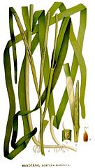
 Enhalus acoroidesmale flowers
 -
 Enhalus acoroidesfemale flowers
 -
-
-

-
-


Seagrass versus seaweed
.png)

"Even though seagrasses and seaweeds look superficially similar, they are very different organisms. Seagrasses belong to a group of plants called monocotyledons that include grasses, lilies and palms. Like their relatives, seagrasses have leaves, roots and veins, and produce flowers and seeds. Chloroplasts in their tissues use the sun's energy to convert carbon dioxide and water into sugar and oxygen for growth through the process of photosynthesis. Veins transport nutrients and water throughout the plant, and have little air pockets called lacunae that help keep the leaves buoyant and exchange oxygen and carbon dioxide throughout the plant. Like other flowering plants, their roots can absorb nutrients. Unlike flowering plants on land, however, they lack stomata—the tiny pores on leaves that open and close to control water and gas exchange. Instead, they have a thin cuticle layer, which allows gasses and nutrients to diffuse directly into and out of the leaves from the water. The roots and rhizomes (thicker horizontal stems) of seagrasses extend into the sediment of the seafloor and are used to store and absorb nutrients, as well as anchor the plants. In contrast, seaweeds (algae) are much simpler organisms. They have no flowers or veins, and their holdfasts simply attach to the bottom and are generally not specialized to take in nutrients. Scientists are studying what genes were lost and which were regained as seagrasses evolved from algae in the sea to plants on land, and then transitioned back to the sea. The entire genome of one seagrass, the eelgrass Zostera marina, was sequenced in 2016, helping us understand how these plants adapted to life in the sea, how they may respond to climate warming, and the evolution of salt tolerance in crop plants."[12]
Evolution
- Les DH, MA Cleland and M Waycott (1997) "Phylogenetic studies in Alismatidae, II: evolution of marine angiosperms (seagrasses) and hydrophily" Systematic Botany, 22 (3): 443–463.
- Waycott M, Procaccini G, Les DH and Reusch TBH (2006) "Seagrass Evolution, Ecology and Conservation: A Genetic Perspective" In: AWD Larkum, RRJ Orth, CM Duarte (Eds) Seagrasses: Biology, Ecology and Conservation, pp 25–50, Springer. ISBN 9781402029837.
- The origin and evolution of seagrasses Page 4f.
- Evolution of seagrasses
- Wissler L, Codoñer FM, Gu J, Reusch TBH, Olsen JL, Procaccini G and Bornberg-Bauer E (2011) "Back to the sea twice: identifying candidate plant genes for molecular evolution to marine life" BMC Evolutionary Biology, 11 (8).
- Algae vs. Plants
Threatened species
"In a recent study, 15 of the 72 known species of seagrasses were listed as 'Endangered', 'Vulnerable' or 'Near Threatened' on the International Union for Conservation of Nature (IUCN) Red List."[4][5]
"Seagrass researcher at the University of Technology Sydney, Peter Macreadie says there are multiple factors that make seagrass vulnerable, but the biggest threat is the creation of anoxic dead zones by algal blooms. “Seagrass are plants that grow on the seafloor, so when nutrient runoff is taken up by the algae, the algae become dense and it blocks the sunlight from reaching the seagrass.” There is also direct damage done by humans via dredging or by boat propellers. If some plants are disturbed in the middle of a meadow, the ‘hole’ will actually get bigger and bigger, eating away the meadow from the inside. “We know we’ve lost 30% of the world’s sea grasses already,” says Macreadie.Many seagrass scientists are now concerned about changes in water temperature caused by the apparent effects of climate change, he added. “Seagrass is changing its range and distribution, but they can only tolerate a certain set of temperatures.” [6]
"Past director of the University of Western Australia’s Oceans Institute, Gary Kendrick says restoration can get expensive. “I’ve been working on a five-year restoration project and the chances of full recovery are still slim, as restoration is high risk and high expenditure. The seagrass restoration itself can cost anywhere from AU$8,000 a hectare to hundreds of thousands of dollars per hectare,” he says. “There are studies of a field that cost $1 million a hectare to restore. That’s about ten times what it costs to restore a forest. It is much easier to conserve the seagrass habitats we already have in the first place, rather than trying to restore them after the fact"[7]
- Hughes AR, Williams SL, Duarte CM, Heck KL and Waycott M (2008) "Associations of concern: declining seagrasses and threatened dependent species" Frontiers in Ecology and the Environment, 7 (5): 242–246.
References
- ^ Seagrasses: Prairies Of The Sea
- ISBN 9781402029837.
- ISBN 9780444874030.
- ISBN 9780520240476. Full text
- ISBN 9781402038808.
- ^ Seagrasses Australian Institute of Marine Science. Retrieved 12 October 2013.
- ^ D. H Les, M. A Cleland, M Waycott, Phylogenic studies in the Alismatidea, II: Evolution of the marine angiosperm (seagrasses) and hydrophily. Systematic Botany 199722443
- ^ Devault, A. Damien and Hélène Pascaline (2013) "Herbicide Impact on Seagrass Communities"
- ^ 'Oldest living thing on earth' discovered The Telegraph, 7 February 2012.
- ^ Maggy Wassilieff. 'Estuaries - Plants of the estuary', Te Ara - the Encyclopedia of New Zealand, updated 9-Jul-13 URL: http://www.TeAra.govt.nz/en/photograph/4624/seagrass
- ^ [1]
- ^ a b Reynolds PL (2018) "Seagrass and Seagrass Beds" Smithsonian Ocean Portal.
Seagrass meadows 2
- Threats to Sharks Destabilize Entire Ecosystems - role of seagrass
Herbivore abundance

As habitats for other species
As a nursery
Earth Times, 10 September 2012.</ref>

Ecosystem services
- Manatee grassis found in shallow brackish offshore areas close to a freshwater outlet.
- likewise turtlegrass
And a critical service for contemporary times, "they capture carbon from the atmosphere and store it in sediments at a rate of about thirty times faster than a tropical rainforest, which are the most powerful carbon sinks on land. and here’s what’s really unique about this seagrass ecosystems, they can store that carbon for thousands of years. A question is, as we lose seagrass beds, what happens to that carbon and how might it affect global climate change?"
"although sea grasses occupy only went 1 percent of the seafloor they are responsible for 11 percent of the organic carbon buried in the ocean their role in the carbon cycle greatly aids in reducing greenhouse gases in the atmosphere"
"Seagrass meadows have as much leaf area as towering rain forests which have the highest sleep areas on the planet seagrass Meadows are more productive than fertilized cornfields a productive seagrass meadow will fizz with oxygen bubbles looking like champagne"
Coastal protection
"Seagrass meadows are hidden underwater grass fields that protect the coast and offer shelter to many sea creatures. Seagrasses are flowering plants that evolved from the land back to the sea, and they now occupy the sea bottom in shallow waters along the coast all over the world. Human activities, such as fishing methods that rely on heavy nets that are dragged across the sea floor, put this important ecosystem at serious risk. In this study, we aimed to measure how seagrasses contribute to coast protection by trapping rock debris transported by the sea. Seagrasses reduce erosion of the coast and protect our houses and cities from both the force of the sea and from sea-level rise caused by global warming. Seagrasses do this by softening the force of the waves with their leaves, and helping sediment transported in the seawater to accumulate on the seafloor."[5]
"they also act as they are to reduce erosion and in that they can actually slow down the movement of water especially during episodic events like hurricanes and storms one of the big things of serious bird does is that the leaves act as baffles in the water so they slow down water movement and encourage particulate matter to settle out so it's a good way of clearing up your your water quality in nearshore environments"
"removing suspended sediments from the water this is good in terms of the water quality that a coral reef wants because if you remember a coral reef warms warm clear salty water clear doesn't like suspended material in the water because that block sunlight that's important to the reef as well this removal of suspended sediments from the water column then builds the the shoreline from the bottom up as it were and allows accretion of sediments close to shore so it's one way of maintaining the stability of your coastline there are lots of other parts in particular algae calcareous algae algae that have a carbonate skeleton but are associated with a seagrass bed and when these die and break down these skeletons are eventually won't wash up on shore and that creates the sand a significant portion of sea grasses accumulates on the beach as Beach Coast Detroiters where the deliver carbonate materials that nourished the beach and contribute to June formation although only a few feet high"
Connectivity with other ecosystems
"Tropical mangrove forests, seagrass beds, and coral reefs are among the most diverse and productive ecosystems on Earth. Their evolution in dynamic, and ever-changing environments means they have developed a capacity to withstand and recover (i.e., are resilient) from disturbances caused by anthropogenic activities and climatic perturbations. Their resilience can be attributed, in part, to a range of cross-ecosystem interactions whereby one ecosystem creates favorable conditions for the maintenance of its neighbors. However, in recent decades, expanding human populations have augmented anthropogenic activities and driven changes in global climate, resulting in increased frequencies and intensities of disturbances to these ecosystems. Many contemporary environments are failing to regenerate following these disturbances and consequently, large-scale degradation and losses of ecosystems on the tropical seascape are being observed. This chapter reviews the wealth of available literature focused on the tropical marine seascape to investigate the degree of connectivity between its ecosystems and how cross-ecosystem interactions may be impacted by ever-increasing anthropogenic activities and human-induced climate change. Furthermore, it investigates how disruption and/or loss of these cross-ecosystem interactions may impact the success of neighboring ecosystems and consequently, the highly-valued ecosystem services to which these ecosystems give rise. The findings from this review highlight the degree of connectivity between mangroves, seagrasses and coral reefs, and emphasizes the need for a holistic, seascape-wide research approach to successfully protect and preserve these critically important ecosystems and their associated services for future generations".[6]


- ancient seagrass

"An ancient seagrass that spans up to 15 kilometres and weighs more than 6,000 metric tonnes may be more than 100,000 years old - making it the oldest living organism, Australian researchers have found. But Posidonia oceanica, which occurs only in the Mediterranean and Australian waters, is now under threat from global warming, the team reported. The seagrass reproduces by asexually generating clones of itself, so meadows spanning vast areas of the seabed are genetically identical and counted as one organism."[10]
Blue carbon

"Blue carbon is the carbon captured by the world’s oceans and represents more than 55% of the green carbon. The carbon captured by living organisms in oceans is stored in the form of sediments from mangroves, salt marshes and seagrasses. It does not remain stored for decades or centu- ries (like for example rainforests), but rather for millennia... the coastal ocean also contains vast areas covered by algal beds. Most macroalgal beds (including kelp forests) do not bury carbon, as they grow on rocky substrates where burial is impossible.... For instance, es- timates of the area covered by mangroves, probably the best constrained amongst vegetated coastal habitats, ranges from 0.11 to 0.24 million sq km (Bouillon et al., 2008). Estimates of the area covered by seagrass meadows, the least constraint estimate, range from a documented area of 0.12 million sq km (Green and Short, 2003), to an upper estimate of 0.6 million sq km (Duarte and Chiscano, 1999) as the South East Asian archipelagos, such as Indonesia, are likely to hold vast, un- charted seagrass meadows (Duarte et al., 2009). Indeed, the coastal area with sufficient submarine irradiance as to support seagrass meadows has been estimated at 5.2 million sq km (Gattuso et al., 2006). Hence, a thorough inventory of blue carbon sinks may well yield a cover twice as large as the mean area considered in current, conservative global assessments (Table 1)... Restoring lost seagrass meadows is more complex, as the labour required to insert transplants under the water in- creases cost. Seagrass restoration projects have consequently remained comparatively limited in size (a few hectares) and number. However it is a viable option provided the benefits of seagrass restoration can be used strategically, for example to catalyze the great potential for natural recovery.... The ocean’s vegetated habitats, in particular mangroves, salt marshes and seagrasses, cover <0.5% of the sea bed. These form earth’s blue carbon sinks and account for more than 50%, perhaps as much as 71%, of all carbon storage in ocean sediments. They comprise only 0.05% of the plant biomass on land, but store a comparable amount of carbon per year, and thus rank among the most intense carbon sinks on the planet.... Vegetated coastal habitats – mangrove forests, saltmarshes and seagrass meadows – have much in common with rain forests: they are hot spots for biodiversity, they provide important and valuable ecosystem functions, including a large carbon sink capacity, and they are experiencing a steep global decline (Duarte et al., 2008, Duarte, 2009). Indeed, the world is losing its coastal habitats four times faster than its rain forests (Duarte et al., 2008, Duarte, 2009) and the rate of loss is accelerating (Waycott et al., 2009). However, whereas society is well informed of the benefits and threats associated with rainforests, there is a comparative lack of awareness on the status and benefits of vegetated coastal habitats. This is perhaps because of a “charisma” gap, where these often submerged, out of sight coastal habitats, are not as appealing to the public as their terrestrial counterparts (Duarte et al., 2008). ... The remaining excess production of mangrove forests, salt-marshes and sea- grass meadows is buried in the sediments, where it can remain stored over millenary time scales (Mateo et al., 1997), thereby representing a strong natural carbon sink. This is most evident in the case of seagrass meadows, which accumulate enough materials as to significantly raise the seafloor, forming mats that can exceed 3 metres in depth. In addition to burying a fraction of their own production, blue carbon sinks reduce flow, alter turbulence and attenuate wave action (Koch et al., 2006), thereby promoting sedimentation and reducing sediment resuspension (e.g. Gacia and Duarte, 2001). Recent research has shown that the canopies of seagrass meadows trap particles entrained in the flow, which lose mo- mentum upon impacting on the leaves, thereby promoting the sedimentation of suspended material to the seafloor (Hendriks et al., 2007). Isotopic analyses of the organic carbon accumu- lated in sediments of vegetated coastal habitats have shown that a significant fraction derives from plankton (Gacia et al., 2002).... they are disappearing faster than anything on land and much may be lost in a couple of decades. These areas, covering features such as mangroves, salt marshes and seagrasses, are responsible for capturing and storing up to some 70% of the carbon permanenty stored in the marine realm.... A recent assessment indicates that about one-third of the glob- al seagrass area has been already lost, and that these losses are accelerating, from less than 0.9% year–1 in the 1970’s to more than 7% year–1 since 2000 (Waycott et al., 2009)....".[12]
"We are really only just starting to discover the exact amounts of CO2 released. Linwood Pendleton of Duke University, North Carolina has produced a paper, [http://www.plosone.org/article/info%3Adoi%2F10.1371%2Fjournal.pone.0043542 "Estimating Global "Blue Carbon" Emissions from Conversion and Degradation of Vegetated Coastal Ecosystems", with a large group of fellow-scientists which elucidates this large calculation. While these coastal strips cover 6% of the earth's forests, they make up a massive 20% of the deforestation carbon... The marginal value of damage from climate change that can be caused by one ton of carbon in the atmosphere in 2020 is one heck of an estimate, but it comes out at $41."Cite error: A <ref> tag is missing the closing </ref> (see the help page).
"Seagrass ecosystems contain globally significant organic carbon (C) stocks. However, climate change and increasing frequency of extreme events threaten their preservation. Shark Bay, Western Australia, has the largest C stock reported for a seagrass ecosystem, containing up to 1.3% of the total C stored within the top metre of seagrass sediments worldwide. On the basis of field studies and satellite imagery, we estimate that 36% of Shark Bay’s seagrass meadows were damaged following a marine heatwave in 2010/2011. Assuming that 10 to 50% of the seagrass sediment C stock was exposed to oxic conditions after disturbance, between 2 and 9 Tg CO2 could have been released to the atmosphere during the following three years, increasing emissions from land-use change in Australia by 4–21% per annum. With heatwaves predicted to increase with further climate warming, conservation of seagrass ecosystems is essential to avoid adverse feedbacks on the climate system."[13]
Carbon sequestration
- As a carbon sink
"Estuarine and coastal ecosystems (ECEs) are the most productive marine ecosystems and provide the diverse and valuable functions and services. Because ECEs are the ‘open’ systems strongly connected with both the land and ocean, the connectivity and interactions across land–ocean gradients determine ecosystem structure, functions and processes." [8]
"Coastal vegetated ecosystems are major organic carbon (OC) and total nitrogen (TN) sinks, but the mechanisms that regulate their spatial variability need to be better understood. Here we assessed how superficial sedimentary OC and TN within intertidal vegetated assemblages (saltmarsh and seagrass) vary along a flow gradient, which is a major driver of sediment grain size, and thus of organic matter (OM) content. A significant relationship between flow current velocity and OC and TN stocks in the seagrass was found, but not in the saltmarsh. OC and TN stocks of the saltmarsh were larger than the seagrass, even though that habitat experiences shorter hydroperiods. ... Blue carbon designates the carbon stored and sequestered in marine ecosystems, particularly vegetated coastal systems including seagrasses and saltmarshes1. These ecosystems are of global importance for sequestering atmospheric carbon dioxide2,3, yet the global decline of seagrasses4 and saltmarshes5 is not only reducing this important natural carbon sink but may cause the release of the captured carbon dioxide back to the atmosphere6,7,8,9,10,11. For these reasons, the protection and restoration of coastal vegetated ecosystems have been recognized as key global strategies in climate change mitigation12. The blue carbon field has grown rapidly in the last years with the aim of getting better estimations of carbon stocks in coastal vegetated ecosystems and their role in the ocean carbon budget13,14. However, the understanding of the mechanisms regulating the spatial variability of the organic carbon stocks in costal vegetated ecosystems remains limited15."[14]
"Seagrass meadows are considered important natural carbon sinks due to their capacity to store organic carbon (Corg) in sediments. However, the spatial heterogeneity of carbon storage in seagrass sediments needs to be better understood to improve accuracy of Blue Carbon assessments, particularly when strong gradients are present. We performed an intensive coring study within a sub-tropical estuary to assess the spatial variability in sedimentary Corg associated with seagrasses, and to identify the key factors promoting this variability. We found a strong spatial pattern within the estuary, from 52.16 mg Corg cm−3 in seagrass meadows in the upper parts, declining to 1.06 mg Corg cm−3 in seagrass meadows at the estuary mouth, despite a general gradient of increasing seagrass cover and seagrass habitat extent in the opposite direction. The sedimentary Corg underneath seagrass meadows came principally from allochthonous (non-seagrass) sources (~70–90 %), while the contribution of seagrasses was low (~10–30 %) throughout the entire estuary. Our results showed that Corg stored in sediments of seagrass meadows can be highly variable within an estuary, attributed largely to accumulation of fine sediments and inputs of allochthonous sources... Seagrass ecosystems are among the most significant natural carbon sinks worldwide, since they can sequester significant amounts of carbon, store it as organic carbon (Corg) in the sediments for long periods of time, and have a worldwide distribution1,2,3. It is estimated that seagrass ecosystems store globally up to 19.9 petagrams (Pg) of Corg in sediments2, or between 4.2 and 8.4 Pg of Corg from a more conservative approach2, where Corg could be stored in sediments for hundreds of years and even millennia4."[15]
"In nearly all the seas around the world, in the shallow waters next to the land, are secret underwater gardens. These gardens are home to a special marine (saltwater) plant called seagrass. When seagrass grows in large areas, the habitat it creates is called a seagrass meadow. Seagrass meadows play an important role in keeping our oceans healthy and providing a home for all kinds of marine life. This marine life includes fishes that people eat, such as cod and plaice but also endangered species such as seahorses, turtles, and sea cows. Seagrasses absorb large amounts of carbon dioxide from the surrounding seawater, and so help to reduce the speed of climate change. Seagrasses help protect our coastlines from storms and rising tides because their leaves take energy out of the waves hitting the coast, and their roots act as an anchor in the underwater sand. Seagrasses also soak up nutrients and bacteria, helping to keep our seawater clean. But seagrasses around the world are being lost at a rate of about two football fields every hour. Lots of things can damage seagrass, from polluted water to boats dragging their anchors in seagrass meadows. Overfishing is a problem, since it causes an imbalance in the food chain. Unfortunately, seagrass does not get the attention it deserves because most people are unaware of its existence. We need to increase awareness of the importance of this beautiful and valuable habitat and get more people involved in monitoring and protecting seagrass, before it is too late."[16]
"Carbon captured by marine living organisms is called “blue carbon”, and seagrass meadows are a dominant blue carbon sink. However, our knowledge of how seagrass increases sedimentary organic carbon (OC) stocks is limited. We investigated two pathways of OC accumulation: trapping of organic matter in the water column and the direct supply of belowground seagrass detritus."[17]
"sea grass has helped to sustain human life in a variety of waves over a billion people live within 30 miles of a seagrass meadow millions of people obtain their protein from animals that live in sea grasses the grasses have been used by humans for over ten thousand years a lot of the seagrass is used in furniture in our firm stunts the stuff cushions and make beds so it's not just a fishery thing it's not just the coastline thing but it is right throughout the fabric of your coastal population tropical sea grasses in the Caribbean are among the most productive in the world it's very important in terms of productivity the same function on land where plants during the day photosynthesize and produce oxygen produce biomass and export this biomass to other ecosystems to be consumed by other animals and plants because of the breakdown of nutrients same thing happens in the water so that you have a lot of reef fish for instance that come in to prey on other species that as juveniles are found only in seagrass beds or in nearby mangrove systems and there's this interplay of species interdependence of species the sea grasses are very important nursery habitats so they actually support the overall fishery that's associated with the coastal environments this productivity of course is reflected in the extensive fishery resources that's associated with coastal environments where they are found we have fish for example the grunt and the snappers we have spiny lobsters combs they are the primary food source for the world's largest marine herbivores the West Indian manatee and the dugong are a major food source of green sea turtles "
Accelerating loss
- Accelerating loss of seagrasses across the globe threatens coastal ecosystems (cited by 2579)
"Coastal ecosystems and the services they provide are adversely affected by a wide variety of human activities. In particular, seagrass meadows are negatively affected by impacts accruing from the billion or more people who live within 50 km of them. Seagrass meadows provide important ecosystem services, including an estimated $1.9 trillion per year in the form of nutrient cycling; an order of magnitude enhancement of coral reef fish productivity; a habitat for thousands of fish, bird, and invertebrate species; and a major food source for endangered dugong, manatee, and green turtle. Although individual impacts from coastal development, degraded water quality, and climate change have been documented, there has been no quantitative global assessment of seagrass loss until now. Our comprehensive global assessment of 215 studies found that seagrasses have been disappearing at a rate of 110 km2 yr−1 since 1980 and that 29% of the known areal extent has disappeared since seagrass areas were initially recorded in 1879. Furthermore, rates of decline have accelerated from a median of 0.9% yr−1 before 1940 to 7% yr−1 since 1990. Seagrass loss rates are comparable to those reported for mangroves, coral reefs, and tropical rainforests and place seagrass meadows among the most threatened ecosystems on earth."[18]
"Seagrass ecosystems face widespread threat from reduced water quality, coastal development and poor land use. In recent decades, their distribution has declined rapidly, and in the British Isles, this loss is thought to have been extensive. Given increasing knowledge of how these ecosystems support fisheries production, the understanding of their potential rapid loss, and the difficulty in restoring them, it is vital we develop an understanding of the risks they are under, so that management actions can be developed accordingly. Developing an understanding of their environmental status and condition is therefore critical to their long-term management. This study provided, to our knowledge, the first examination of the environmental health of seagrass meadows around the British Isles..."[19]
"in June 2009 an international team of scientists warned that accelerating losses of sea grasses across the globe threatens the immediate health and long-term sustainability of coastal ecosystems the team found that approximately 58 percent of the world's seagrass meadows are currently declining an estimates that sea grasses have been disappearing at the rate of around 110 square kilometers per year since 1980, They cite two primary causes for the decline: direct impact from coastal development and dredging activities and the indirect impact of declining water quality. The tendency is once you build in the coastal zone in an irresponsible manner it means that some of your waste material is going to be going to end up in the ocean so in building as well you will tend to clear mangrove swamps and mangrove swamps act as natural filters now once you get pollutants going into the ocean and once you get a heavy sediment load because we win will naturally come and when do we enforce and earth is going to pick up material as it goes now if that material gets out into the ocean is going to smother the seagrass there are plants they photosynthesize they depend on sunlight to live now if there's a heavy sediment load lots of sediment in the water the sunlight is not going to penetrate down to the seagrass and without sunlight plants cannot live."
Seagrass restoration
"Seagrasses provide multiple ecosystem services including nursery habitat, improved water quality, coastal protection, and carbon sequestration. However, seagrasses are in crisis as global coverage is declining at an accelerating rate. With increased focus on ecological restoration as a conservation strategy, methods that enhance restoration success need to be explored. Decades of work in coastal plant ecosystems, including seagrasses, has shown that positive species relationships and feedbacks are critical for ecosystem stability, expansion, and recovery from disturbance. We reviewed the restoration literature on seagrasses and found few studies have tested for the beneficial effects of including positive species interactions in seagrass restoration designs. Here we review the full suite of positive species interactions that have been documented in seagrass ecosystems, where they occur, and how they might be integrated into seagrass restoration. The few studies in marine plant communities that have explicitly incorporated positive species interactions and feedbacks have found an increase in plant growth with little additional resource investment. As oceans continue to change and stressors become more prevalent, harnessing positive interactions between species through innovative approaches will likely become key to successful seagrass restoration."[11]

from youtube clip
"Seagrass is another critically important habitat as far as coral reefs and general ocean health is concerned. You’ve got the coral reefs, it’s so obvious they’re beautiful, there’s fish around them. but you look at seagrass and most people actually don’t like it. you don’t like walking on the seagrass. you like bare sand, crystal clear water."[9]
Seagrasses evolved from flowering land plants about 100 million years ago. As plants, they retain in the ocean many of the behaviours they had on land. They flower and reproduce by producing male and female gametes that fertilise each other in the water. They can also reproduce asexually by budding or cloning themselves.
Altogether, there are only about 60 species of sea grasses. They colonise sea coast around the world, apart from polar regions. Protected bays and estuaries often shelter extensive seagrass meadows. In tropical regions, sea grasses often colonise the area between beaches and reefs. The species mix of seagrasses changes according to how tropical or temperate the region is.
Seagrasses are declining in many areas. Prior to a decline it has been noticed that the algae that normally grow on the blades of seagrasses become much more abundant. There algae are called epiphytes.
"Pollutants getting into the ocean they can have a direct toxic effect on the seagrass another indirect effect pollutants can have and when I say pollutants I don't mean necessarily the nasty chemicals a simple thing as fertilizer that you apply to your lawn and golf post is in the coastal area they gets washed down into the ocean those fertilizers they fertilize on land they also fertilize certain things in the water algae will use that fertilizer and you'll get what we call a bloom an explosion in goo in these algae once that explosion occurs it will tend to block out sunlight as well these algae some of them can produce toxins which actually poison everything else in the area sea grasses in the Caribbean face all of these threats there's also switch which is an important factor also illegal Sandman and uh increases their sediment load to the denying environment all of those impact on the sea grasses now sea grasses the government will try to put them protect them from development. [10]
"No coastal development all right, across the Caribbean there's a huge pressure for that because we are a tourism based society so persons we want to make beaches first want to make beachfront properties and other beaches to be unfriendly to your tourist scratching up on their feet and having orgasms like stingrays and jellyfish in the sea grass so they try to remove it so the government for example in Jamaica if you want to do such a development you have to do a serious relocation all the things that that happened is that development of ports there's a lot of dredging activities maintenance dredging of ports with that increased amount of shipping then there's a likelihood of ships running aground propeller scars also damaging the seagrass beds all of this impact under the ecosystem in sea grasses other significant threats include dynamite fishing illegal sand mining and pollution from land-based sources such as hydrocarbons pesticides plastics and other toxic wastes when it comes to sea grasses as well as all other marine ecosystems important thing about them is to protect them in however we can the government tries to put in laws and regulations however what are the most important things the tools in protecting these resources is education so no matter what laws exist no matter what sanctions you put against people if you educate persons as to the importance of these ecosystem then a more likely to try to protect them for example you might see other you might see breaches occurring across a be like this know if somebody hears and know what shouldn't be done then there be inclined to report this breach so education in school is paramount to the success of any coastal management plan. [11]
"when it comes to sea grasses even though they're not as attractive as coral reefs the thing with seagrass is that there's a lot more things that you cannot see for example you have organisms and crusting on the blades and there are thousands of organisms there which we cannot see and not to mention the vast amounts of carbon diseased plants can convert to oxygen on a daily basis it's basically comparable to the phytoplankton and the sea which makes most of our oxygen the rules that it provides our management strategies have to be diverse and education as well as the local laws have to be very important in that information is at the center of a successful coastal zone management strategy each country must acquire and maintain an inventory of its coastal environments and resources in Jamaica we do mapping I know some other islands no change that for example does some amount of mapping quite sure about all the rest of the islands but it is important to do mapping to see where your resources are so that when development comes along you don't know where I know what the potential impacts will be so it helps you to better manage your a coastline so once you have the mapping you have that in venture especially in a GIS format so that once some development comes along then it can play still address to see what error will be destroyed or disturb and what is a potential impact so the discover Bay Marine Laboratory in addition to the Port Royal Marine Lab which is a part of university West Indies we have for over 50 years in very instrumental in doing research on these different coastal ecosystems in addition to educational programs reduce a vast amount of outreach not only to high schools but even when it comes to teachers colleges we have teachers learning to the educators in science as well as our primary in elementary school a large amount of education and outreach with them as well the implementation of a successful integrated coastal zone management strategy is dependent on a strong legal and international framework in the end knowledge and cooperation are the keys to protecting sea grasses and other natural wonders of the Caribbean".[12]
"The lowest reaches of an estuary are covered by the sea for all or most of the tidal cycle. Seagrass (at left) is the only plant that can withstand such long immersion in sea water. Mangrove grows further up the shore. Salt meadows, rushes and shore ribbonwood grow on the highest reaches."[13]
Gallery
-
 seagrass (green), oyster reefs (pink), sand bottom (yellow), mangroves (magenta), and salt marsh (light blue)
 -
 A seagrass meadow. Florida Keys National Marine Sanctuary.
 -

-
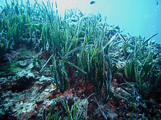
-

-
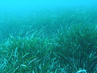
-
seagrass meadow
-
 Healthy seagrass, Florida Keys National Marine Sanctuary
 -
 Seagrass, California, Channel Islands NMS
 -
 Sea grasses near beach along Pacific Ocean
 -
 Sea Grass at rest between tides
 -

-
 Fern seagrasses, Halophila spinulosa, can cover large areas in a green feathery carpet
 -
 Thick seagrass between the shore and a reef
 -

-
 Pipefish and tube snouts among seagrass at Monterey Bay Aquarium
 -
 Seagrass lagoon, Chek Jawa, Pulau Ubin, Singapore.


.jpg)


Sources
- Videos
- Articles
- Can seagrass save the world’s coral reefs?
- Endangered seagrasses can store carbon
- Marine Ecology December 2006 - special issue on seagrasses
- Seagrasses About.com.
- Seagrasses Ichthyology, Florida Museum of Natural History.
- Seagrass meadows Marine Biodiversity Wiki.
- Seagrass Habitats Smithsonian Marine Station at Fort Pierce.
- Global Research to Better Understand Seagrasses in their Environment
- Seagrasses: Prairies of the sea
- Comparing seagrass meadows across New Zealand
- "Accelerating loss of seagrasses across the globe threatens coastal ecosystems"
- Importance of Seagrass
- Seagrass meadows in “hot water” IUCN, 25 July 2008.
- Brasier MD (1975) "An outline history of seagrass communities" Palaeontology, 18: 681–702.
- Duarte, Carlos M (2011) Seagrass meadows Encyclopedia of Earth. Updated: 20 October 2011.
- Seagrasses University of Arizona.
- Guillén, Juan Eduardo (2013) Evolution of Posidonia oceanica seagrass meadows and its implications for management Journal of Sea Research.
- Seagrass Fact Sheet Department of Fisheries, Western Australia.
- Lardizabal, Sarah (2006) Beyond the Refugium: Seagrass Aquaria www.reefkeeping.com
- Seagrass link to seahorse upright posture
- Klumpp DW, Salita-Espinosa J and Fortes M (1993) ["Feeding ecology and trophic role of sea urchins in a tropical seagrass community"] Aquatic Botany, 45 (2–3): 205–229.
- New Study Provides Global Analysis of Seagrass Extinction Risk Science News, 5 June 2011.
- I hate plants, but seagrasses are awesome
- Marine Botany Lecture 16 - Seagrasses
- Seagrasses of South Australia
- Teske, Peter R. and Luciano B. Beheregaray (2009) "Evolution of seahorses' upright posture was linked to Oligocene expansion of seagrass habitats" Biology Letters, 5 (4): 521–523.
- van der Heide T et al.(2012) "A Three-Stage Symbiosis Forms the Foundation of Seagrass Ecosystems" Science, 336 (6087): 1432–1434.
- Three Steps for Seagrass Success
- Seagrasses, Dunes and Salt Marshes
- Short F, Carruthers T, Dennison W, Waycott M (2007) Materials/Habitats/GLOBAL Seagrass distribution.pdf "Global seagrass distribution and diversity: A bioregional model" Journal of Experimental Marine Biology and Ecology, 350: 3–20.
- 1 Ocean and Coastal Habitat - SECTION 5 Sea Grasses.pdf Seagrasses
- Dennison, William C. (2009) Global Trajectories of Seagrasses, the Biological Sentinels of Coastal Ecosystems Fundación BBVA. ISBN 978-84-96515-84-0.
- Boström C, Pittman SJ, Simenstad C and Kneib RT (2011) "Seascape ecology of coastal biogenic habitats: advances, gaps, and challenges" 427: 191–217.
- Modeling Nonlinear Seagrass Clonal Growth: Assessing the Efficiency of Space Occupation across the Seagrass Flora
- Seagrass Phylogeny
- Seagrasses as ecosystem engineers
- "Contribution of genetics and genomics to seagrass biology and conservation"
- {Wave Energy and the Upper Depth Limit Distribution of Posidonia oceanica"
- Bacteria-Mollusc-SeaGrass symbiosis: a tale of ecological interactions
- Failure to protect seagrass may cost Australia $45b
- THE DIVERSITY AND DISTRIBUTION OF SEAGRASS IN SINGAPORE
- Flowering plants in the sea, part 1 - photosynthesis
- Flowering plants in the sea part 2 - Sex
- Seagrass meadows, better than forests
- Two's company, three's community ecology
- Hewitt, Judi (2007) "Does seagrass contribute to marine biodiversity?" Water & Atmosphere, 15 (1) 18–19.
- Seagrass community (chapter)
- Seagrass… It’s Alive!
- Seagrass ‘tens of thousands of years old’ BBC, 2 February 2012.
- Minelli, Alessandro et al. (2008) Seagrass meadows Italian Ministry of the Environment and Territorial Protection. ISBN 88 88192 39 5.
- Essay for November 2012: The seagrass community
- Management and conservation of seagrass in New Zealand: an introduction
- SPECTACULAR PRESERVATION OF SEAGRASSES AND SEAGRASS-ASSOCIATED COMMUNITIES FROM THE PLIOCENE OF RHODES, GREECE
- "Can we predict the future: juvenile finfish and their seagrass nurseries in the Chesapeake Bay"
- Sophie Arnaud-Haond, Carlos M. Duarte, Elena Diaz-Almela, Núria Marbà, Tomas Sintes, Ester A. Serrão. Implications of Extreme Life Span in Clonal Organisms: Millenary Clones in Meadows of the Threatened Seagrass Posidonia oceanica. PLoS ONE, 2012; 7 (2): e30454 DOI: 10.1371/journal.pone.0030454
- Organisations
- Recovery
- Seagrasses – Global Distribution Seagrass Recovery
- Seagrass Recovery
- Sharks help seagrass communities though trophic cascade
- sea otters
- Study finds endangered sea grasses boosted by return of sea otters The Independent, 26 August 2013.
- Sea Otters Promote Recovery of Seagrass Beds
- Lucinidae
- Lucinidae
- Interactions between endosymbiont-bearing infaunal bivalves and the biogeochemistry of Thalassia testundinum sediments" – see Lucinidae
- Dugongs, manatees and seagrass
"Seagrass was an important dietary resource for these animals from early in their evolution, as is evident by the association of sirenian fossils with deposits containing fossilised seagrasses. The sea cows' use of seagrass meadows probably brought about substantial changes in the structure and dynamics of this ecosystem, and it has been suggested that "the close herbivore-plant connection between sirenians and seagrasses over the past 50 million years may have led to significant co-evolution" (Clementz et al. 2006, Journal of Vertebrate Paleontology, vol. 26, p. 365)."[20]
- Reports
- Koch, E.W., L.P. Sanford, S.N. Chen, D.J. Shafer and J.M. Smith (2006) [el.erdc.usace.army.mil/elpubs/pdf/tr06-15.pdf Waves in seagrass systems: review and technical recommendations] US Army Corps of Engineers Technical Report. Engineer Research and Development Center, ERDC TR-06-15.
- Waycott, Michelle et al. (2007) Vulnerability of seagrasses in the Great Barrier Reef to climate change Pages 193–236 of a report by the Great Barrier Reef Marine Park Authority and Australian Greenhouse Office.
- handbook
- Borum, Jens, Carlos M. Duarte, Dorte Krause-Jensen and Tina M. Greve (Eds) (2004) European Seagrasses: an introduction to monitoring and management EU project Monitoring and Managing of European Seagrasses (M&MS) EVK3-CT-2000-00044.
- Books
- Hogarth, Peter (2007) The Biology of Mangroves and Seagrasses Oxford University Press. ISBN 9780198568711.
- Bjork M, Short F, McLeod E and Beer S (2008) Managing Seagrasses for Resilience to Climate Change IUCN. ISBN 9782831710891. Text
- Dawes, Clinton J (1998) Marine Botany John Wiley & Sons. ISBN 9780471192084.
- Hemminga MA and Duarte C (20000 Seagrass Ecology Cambridge University Press. ISBN 9780521661843.
- Karleskint G, Turner RL and Small JW (2009) "Marine+Biology"+Seagrasses&hl=en&sa=X&ei=Lu5UUpzkJYGWiAKixoGQAg&ved=0CDoQ6AEwAg#v=onepage&q="Marine Biology" Seagrasses&f=false Introduction to Marine Biology Cengage Learning. ISBN 9780495561972.
- Larkum AWD, Orth RJ and Duarte CM (2007) Seagrasses: Biology, Ecology and Conservation Springer. ISBN 9781402029837. PDF
- Orth, Robert J. et al. "A Global Crisis for Seagrass Ecosystems" BioScience, 56 (12): 987–996.
- Short FT, Polidoro B, Livingstone SR, Carpenter KE and 22 others (2011) "Extinction risk assessment of the world’s seagrass species" Biological Conservation, 144 (7): 1961–1971.
- Sumich, James L and Morrissey, John Francis (2004) Introduction to the Biology of Marine Life Jones & Bartlett Learning. ISBN 9780763733131.
- Waycott, Michelle et al."Accelerating loss of seagrasses across the globe threatens coastal ecosystems" Proceedings of the National Academy of Sciences, 106 (30): 12377–12381.
- Manuals
- Di Carlo G. and McKenzie L.J. (2011) Seagrass training manual for resource managers Conservation International, USA.
- McKenzie, L.J. (2003) Guidelines for the rapid assessment and mapping of tropical seagrass habitats QFS, NFC, Cairns.
Reports...
- Blue Carbon - The Role of Healthy Oceans in Binding Carbon
- Eveleth, Pose (2010) Seagrass: A potential carbon sink UNEP Report ENVR 102.
Other...
- Families
Zosteraceae|Hydrocharitaceae|Posidoniaceae|Cymodoceaceae
- Genera
Phyllospadix|Zostera|Enhalus|Halophila|Thalassia|Posidonia|Amphibolis|Cymodocea|Halodule|Syringodium|Thalassodendron
- IMAGES...
See also
- Seagrass eel
- Wooramel Seagrass Bank
- Seagrass parrotfish
- Seagrass Blenny
- Pedro Bank
- Ronald C. Phillips
- Florida Keys National Marine Sanctuary
- Seagrasses of Western Australia
- Pulai River
- Lobatus gigas
- Green sea turtle
- Alligator pipefish
- Nursery habitat
- Milk shark
- Striped stingaree
- Indian threadfish
- Blind shark
- Fringing reef
- Spotted stingaree
- Labyrinthula
- Parrotfish
- Bluespotted trevally
- King George whiting
- Tawny nurse shark
- Porcupine ray
- Blacknose shark
- AlgaeBase
- Salt marsh
References
- ^ Díaz, S., Fargione, J., Chapin, F. S., and Tilman, D. (2006). Biodiversity loss threatens human well-being. PLOS Biol. 4:e277. doi: 10.1371/journal.pbio.0040277
- ^ Garcia Rodrigues, J., Conides, A., Rivero Rodriguez, S., Raicevich, S., Pita, P., Kleisner, K., et al. (2017). Marine and coastal cultural ecosystem services: knowledge gaps and research priorities. One Ecosyst. 2:e12290. doi: 10.3897/oneeco.2.e12290
- doi:10.3389/fpls.2018.00127.. Material was copied from this source, which is available under a Creative Commons Attribution 4.0 International License
- doi:10.3390/d12080292.. Material was copied from this source, which is available under a Creative Commons Attribution 4.0 International License
- ^ Cite error: The named reference
Fusi2019was invoked but never defined (see the help page). - ^ doi:10.1007/978-3-319-93284-2_9.. Material was copied from this source, which is available under a Creative Commons Attribution 4.0 International License
- ^ a b Moberg F and Folke C (1999) "Ecological goods and services of coral reef ecosystems". Ecol Econ, 29: 215–233. doi:10.1016/S0921-8009(99)00009-9.
- ^ a b Heck KL, Carruthers TJB, Duarte CM et al (2008) "Trophic transfers from seagrass meadows subsidize diverse marine and terrestrial consumers". Ecosystems, 11: 1198–1210. doi:10.1007/s10021-008-9155-y.
- ^ a b Berkström C, Gullström M, Lindborg R et al (2012) "Exploring “knowns” and “unknowns” in tropical seascape connectivity with insights from East African coral reefs". Estuar Coast Shelf Sci, '107: 1–21. doi:10.1016/j.ecss.2012.03.020.
- ^ 100,000-year-old seagrass could be the world’s oldest organism The Conversation, 7 February 2012.
- ^ doi:10.3389/fmars.2020.00091.. Material was copied from this source, which is available under a Creative Commons Attribution 4.0 International License
- ^ Blue Carbon - The Role of Healthy Oceans in Binding Carbon
- .
- .
- .
- doi:10.3389/frym.2018.00002.. Material was copied from this source, which is available under a Creative Commons Attribution 4.0 International License
- ^ doi:10.5194/bg-15-4033-2018.. Material was copied from this source, which is available under a Creative Commons Attribution 4.0 International License
- .
- doi:10.1098/rsos.150596.. Material was copied from this source, which is available under a Creative Commons Attribution 4.0 International License
- ^ [Agriculture in dugongs] Map of Life, University of Cambridge. Retrieved 13 October 2013.
Sponge spicule
- Overview
"Sponges make up the simplest animal group on the planet: phylum Porifera (from the Latin porus ‘pore’ and ferre ‘to bear’). Having no digestive tract, localized sensory region, or true tissues, they are little more than a cluster of cells supported by a structure of spongin and spicules. Spongin is the flexible material that makes up the body wall of the sponge, while spicules are hard, spiny secretions that help to provide a reinforced structure. The cells lining the inside of the sponge are called choanocytes (‘collar cells’), which have a ‘tail-like’ flagellum. The beating flagella of the choanocytes create water currents that flow through the canals and pores in the sponge, bringing in oxygen and particles of food that are consumed."[1]
"To be classified as a sponge, an organism must have spicules, which are needle-like secretions of calcium carbonate or silica. Spicules are classified based on their structural characteristics and size. Megascleres are large, whereas microscleres are small. The number of axes in a spicule differentiates between being called a monoaxon (one axis), triaxon (three axes), tetraxon (four axes), or polyaxon (many axes). If you think of a plus sign (+), it has two axes; one horizontal and one vertical. The number of crossing lines in a spicule determines how many axes it will have. Spicules can also be described in terms of the number of directions in which they grow. Each pointed end of a spicule signifies a single growth direction, which differntiates between monoactine, diactine, triactine, hexactine, tetracline, and polyactine."[1]
"For example, a toothpick-shaped spicule has only one line (axis) so it would be monoaxon. Since it has two distinct points (growth directions), it would also be called diactine."[1]
"Although the oldest fossil evidence for sponges is firmly rooted in the Cambrian, other evidence suggests an even earlier existence. Possible sponge body fossils has been proposed from the Ediacaran, although poor preservation suggest prevents definitive identifications. Other evidence of biomarkers and loose spicules date further back to the Cryogenian (720-635 million years ago), but without additional evidence, it’s difficult to say if these came from early sponges or rather related single-celled organisms. Watch the video below to learn more about these discoveries!"[1]
"Early stem-group sponges from the Paleozoic are commonly lumped together and called 'Reticulosans'. These sponges have thin walls with hexactine spicules, and many taxa have been placed in this ‘trash bin’ group (meaning that their placement within sponge phylogeny is uncertain). The ambiguous structure of early sponges and poor preservation has made sorting out their early evolution a very difficult process."[1]
"Sponges often become disarticulated soon after death, with only spicules remaining. Therefore, most of the fossil record of non-mineralizing sponges consists of their spicules. There are, however, some body fossils of non-mineralized sponges that are known from lagerstatten deposits."[1]
-
![Diversity of spicule morphology and sets of selected sponge species[2]](//upload.wikimedia.org/wikipedia/commons/thumb/4/49/Diversity_of_spicule_morphology_and_sets_of_selected_sponge_species.jpg/531px-Diversity_of_spicule_morphology_and_sets_of_selected_sponge_species.jpg) Diversity of spicule morphology and sets of selected sponge species[2]
Diversity of spicule morphology and sets of selected sponge species[2] -
![Morphology of gemmuloscleres and spicules of freshwater sponges of the order Spongillida[2]](//upload.wikimedia.org/wikipedia/commons/thumb/7/73/Morphology_of_gemmuloscleres_and_spicules_of_freshwater_sponges_of_the_order_Spongillida.jpg/518px-Morphology_of_gemmuloscleres_and_spicules_of_freshwater_sponges_of_the_order_Spongillida.jpg) Morphology of gemmuloscleres and spicules of freshwater sponges of the order Spongillida[2]
Morphology of gemmuloscleres and spicules of freshwater sponges of the order Spongillida[2] -
![Morphological diversity of selected marine sponge spicules[2]](//upload.wikimedia.org/wikipedia/commons/thumb/7/7c/Morphological_diversity_of_selected_marine_sponge_spicules.jpg/261px-Morphological_diversity_of_selected_marine_sponge_spicules.jpg) Morphological diversity of selected marine sponge spicules[2]
Morphological diversity of selected marine sponge spicules[2]
![Diversity of spicule morphology and sets of selected sponge species[2]](/File:Diversity_of_spicule_morphology_and_sets_of_selected_sponge_species.jpg)
![Morphology of gemmuloscleres and spicules of freshwater sponges of the order Spongillida[2]](/File:Morphology_of_gemmuloscleres_and_spicules_of_freshwater_sponges_of_the_order_Spongillida.jpg)
![Morphological diversity of selected marine sponge spicules[2]](/File:Morphological_diversity_of_selected_marine_sponge_spicules.jpg)
Biomineralisation
ABSTRACT (NOT CC): "Sponges secrete a variety of mineral skeletons consisting of calcite, aragonite, and (or) amorphous silica that confer strength and protect them from physical perturbations. Calcification takes place in a solution of bicarbonate and calcium ions, which is supersaturated with respect to both calcite and aragonite. In contrast, silicaous spicules are formed from an environment that is undersaturated with respect to silicon. Silification is the predominant process of biomineralization in extant sponges (92% of the species). The number of axes of symmetry in the large skeletal elements (megasclere spicules) is the main skeletal difference between the classes Hexactinellida (monaxons and triaxons) and Demospongiae (monaxons and tetraxons). Hypersilification occurs in both lithistid demosponges and hexactinellids, which are mostly confined to silicon-rich environments. Both siliceous and calcareous sponge skeletons are deposited within a well-defined restricted space by the so-called matrix-mediated mineralization. Both processes require organic molecules, which are secreted by a particular cell type (sclerocytes) and guide spicule formation. In most siliceous sponges, these molecules form a discrete filament, which is mainly triangular or quadrangular in cross section in demosponges and hexactinellids, respectively. No discrete axial filament has been reported for calcareous sponges. Silica polycondensation produces nanospheres to microspheres, which are arranged in concentric layers to form the spicules. The potential number of silicaous spicule types in a sponge species appears to be fixed genetically, but the environmental conditions (specifically the availability of silicon) may determine whether a genetically determined spicule type is finally expressed."[3]
Biomineralisation 2
Calcareous sponges are the only sponges that form calcitic spicules, which, based on the number of rays (actines) are distinguished in diactines, triactines and tetractines. Each actine is formed by only two cells, called sclerocytes.[4]
By the process of biomineralization many animal groups produce mineral structures like skeletons, shells and teeth. Biominerals differ in shape considerably from their inorganic mineral counterparts1. In order to build specific skeletal structures, organisms have to control the biomineralization process. This control involves proteins with different functions. For calcium carbonate biominerals, which are the most widespread minerals formed by animals2, the directional transport and accumulation of inorganic ions to the calcification site is achieved by specialized transporters, i.e. by bicarbonate transporters (BCTs) or Ca2+-transporters e.g., refs 3 and 4. Linked to bicarbonate transport and pH-regulation is the catalytic activity of carbonic anhydrases (CAs), which catalyse the reversible reaction of CO2 to bicarbonate5. Specialized CAs are key biomineralization proteins in calcium carbonate producing animals6. In addition, proteins of the skeletal organic matrix (SOM) have been identified by means of proteomics, transcriptomics and genomics7. Skeletal proteomes comprise mostly secreted proteins, and often include acidic proteins with high proportions of the amino acids aspartic acid or glutamic acid7,8. These acidic SOM proteins presumably interact with the calcium carbonate crystals and thereby can influence the growth and shape of biominerals9. However, little is known how the expression of biomineralization genes is coordinated and influences the biomineral shape.[4]
Calcareous sponges (Porifera, class Calcarea) are an ideal system to address this question. Their calcite spicules are relatively simple structures, which can be distinguished by the number of their rays (actines) in monaxonic diactines (initially growing in two directions), three-rayed triactines, and four-rayed tetractines10 (Fig. 1A). They are produced by only a few specialized cells, the sclerocytes, often within just a few days11,12. The spicules are growing within an extracellular space, sealed by septate junctions between the membranes of the sclerocytes13,14, and are surrounded by an organic sheath that is secreted by the sclerocytes14. Each spicule is formed by two (diactines), six (triactines) or seven (tetractines) sclerocytes, of which one (termed founder cell) promotes tip growth, and the other, at least in some species, thickens the spicule (the thickener cell)15,16 (Fig. 1B,C). Each founder and thickener cell pair originates from the division of a precursor cell; in case of triactine sclerocytes, these precursors form triplets before they divide14,15,16.[4]
References
- ^ a b c d e f Pier, J. Q. (2019) "Porifera" Digital Atlas of Ancient Life, Paleontological Research Institution, New York. Updated: 16 Sept 2020.
- ^ a b c Cite error: The named reference
Łukowiak2020was invoked but never defined (see the help page). - doi:10.1139/z06-032.)
{{cite journal}}: Cite journal requires|journal=(help); Missing or empty|title=(help - ^ PMID 28406140.. Material was copied from this source, which is available under a Creative Commons Attribution 4.0 International License
Sponge evolution sources
Background
- FROM: Pier, J. Q. (2019) "Porifera" Digital Atlas of Ancient Life, Paleontological Research Institution, New York. Updated: 16 Sept 2020.
- Overview
"Sponges make up the simplest animal group on the planet: phylum Porifera (from the Latin porus ‘pore’ and ferre ‘to bear’). Having no digestive tract, localized sensory region, or true tissues, they are little more than a cluster of cells supported by a structure of spongin and spicules. Spongin is the flexible material that makes up the body wall of the sponge, while spicules are hard, spiny secretions that help to provide a reinforced structure. The cells lining the inside of the sponge are called choanocytes (‘collar cells’), which have a ‘tail-like’ flagellum. The beating flagella of the choanocytes create water currents that flow through the canals and pores in the sponge, bringing in oxygen and particles of food that are consumed."[5]
"Sponges encompass a vast diversity of asymmetrical shapes, sizes, and even hardnesses (ranging from soft and flexible to rock-hard). They have a global distribution, occupy shallow to deep water conditions, and occur in virtually all marine and freshwater environments. In this chapter we will explore the diversity and fossil record of phylum Porifera."[5]
-
![Sponge cells and spicule[5]](//upload.wikimedia.org/wikipedia/commons/thumb/b/bc/Sponge_cells_and_spicule.png/534px-Sponge_cells_and_spicule.png) Sponge cells and spicule[5]
Sponge cells and spicule[5]
![Sponge cells and spicule[5]](/File:Sponge_cells_and_spicule.png)
- Phylogeny
"Being the oldest animal group, sponges have had the longest opportunity to diversify and evolve, which makes their phylogeny rather complex to sort out. Contrary to some early molecular work that suggested that sponges might be paraphyletic, there is a growing consensus that sponges represent a monophyletic group, with the Silicea (a clade that includes the sister taxa Demospongiae and Hexactinellida) sharing a common ancestor with Calcarea and Homoscleromorpha. However, this is continuously under debate and you should consult the recent literature to determine what standing is most current."[5]
- General Features of Sponges
"Sponges are morphologically simple and their basic features are labeled in the image below. Although most of these features are characteristics of all classes, some have become specialized for certain environments."[5]
"If you were to pick up a kitchen or bath sponge, you would feel its soft flexible structure. This soft texture corresponds with the spongin of a living sponge. Although modern kitchen and bath sponges are now made of synthetic materials, living sponges were once collected for human use. The holes throughout the sponge are called ostia, which help channel water flow (containing of food particles) through the sponge. The large openings at the top of a sponge are called oscula, which expels the filtered water and waste out of the sponge."[5]
"Osculum: (oscula, plural) large opening at the top of the sponge where water is expelled Ostia: pores in the body wall Spongin: a flexible protein that makes the soft ‘body’ of the sponge"[5]
"Sponges have developed several body plans of increasing complexity. Ascon grade is the simplest form of pores connecting to a choanocyte-lined internal chamber. Sponges of intermediate complexity are of sycon grade. Although the basic structure is still the same, choanocytes line several incurrent canals, creating more surface area for filter feeding and generation of stronger currents. The most complex structure is leucon grade, where thick walls house an intricate network of canals connecting several flagellated chambers. Although modern calcareous sponges are the only living groups with ascon and sycon grades, they are common fossil forms."[5]
"Sponges also have several microscopic features that are more difficult to see with the naked eye. Most cells in a sponge are totipotent, meaning they can move around and change function throughout their lifetime. They essentially act as stem cells and switch to different forms when needed. Sponges have several kinds of specialized cells that carry out specific life tasks. Check out the video below to see different sponge cells in action!"[5]
"Archaeocytes: amoeboid cells that ingest/digest food particles and transport nutrients to other cells Choanocytes: or ‘collar cells’ are flagellated cells in the body wall, which create currents to capture food particles Pinacocytes: cells that create an outer covering of the sponge, like ‘skin’ Sclerocytes: cells that secrete spicules Spongocytes: cells that secrete spongin Mesohyl: cell layer between the choanocytes and external/internal body wall of sponge, this is where skeletal elements are produced and gametes are stored by many sponge cell types"[5]
- Ocean Filters
"Sponges may have been the first ever ecosystem engineers, meaning they drastically changed the environment around them in a beneficial way. Being such efficient filters, they cleanse the water around them and help cycle nutrients through the water for other living organisms to take advantage of."[5]
"J. Keith Rigby explains “…a black loggerhead sponge, 50cm in diameter and 30cm tall, may draw approximately 1000 L of water through its canal systems in a single day. Other sponges may pass 10,000 to 20,000 times as much water as their volume through their canals in a single day” (Boardman, Cheetham, and Rowell, 1987, p. 132)."[5]
- Symbiosis
"Many sponges are symbiotic, meaning they have physically close, long-term relationships with other organisms. These include many microorganisms such as bacteria, microalgae, archaea, cyanobacteria, and fungi. Some species can house bacteria in their mesohyl, which eat other potentially infectious microorganisms and other things that could make the sponge sick. In deep sea environments other symbionts may be used for chemosynthesis to provide extra nutrition and energy (Hentschel et al., 2002)."[5]
"Sponges are a source of protection and housing for a variety of larger organisms including chordates such as fish and many invertebrates. One species of crab that is informally known as the ‘sponge crab’ will hold a piece of sponge on its back until it attaches to provide extra camouflage."[5]
- Fossil Record
"Studying the early evolution of multicellular animals has been a focal point of research for biologists and paleontologists alike. Sponges are important for understanding this transition. Their primitive nature lacks most distinguishing animal features and their choanocyte cells resemble several features of single-celled eukaryotes, possibly indicating the transition from a cell colony to a multicellular organism. Choanocytes essentially act as stem cells for sponges in that they provide essential life functions, such as acquiring food, but also create the ability to reproduce through gamete production. New developments in gene sequencing and DNA extraction are consistently illuminating our knowledge of how these transitions evolved and further developed."[5]
"Although the oldest fossil evidence for sponges is firmly rooted in the Cambrian, other evidence suggests an even earlier existence. Possible sponge body fossils has been proposed from the Ediacaran, although poor preservation suggest prevents definitive identifications. Other evidence of biomarkers and loose spicules date further back to the Cryogenian (720-635 million years ago), but without additional evidence, it’s difficult to say if these came from early sponges or rather related single-celled organisms. Watch the video below to learn more about these discoveries!"[5]
"Early stem-group sponges from the Paleozoic are commonly lumped together and called 'Reticulosans'. These sponges have thin walls with hexactine spicules, and many taxa have been placed in this ‘trash bin’ group (meaning that their placement within sponge phylogeny is uncertain). The ambiguous structure of early sponges and poor preservation has made sorting out their early evolution a very difficult process."[5]
"Sponges often become disarticulated soon after death, with only spicules remaining. Therefore, most of the fossil record of non-mineralizing sponges consists of their spicules. There are, however, some body fossils of non-mineralized sponges that are known from lagerstatten deposits."[5]
"Soon after the Cambrian explosion, evidence for early members of at least three sponge classes arose. Below is a chronological list of when major sponge groups originated, which you can read more about in the following sections."[5]
"Archaeocyatha, a cryptic sponge clade, became major reef builders during their brief existence in the Early Cambrian. You can learn more about them in the next section! Demospongiae, Hexactinellida, and Calcarea, three of the current sponge classes, all evolved within the Cambrian period. Stromatoporoids arose during the Ordovician and were the second group (after Archaeocyatha) to form reefs; they were especially important reef builders during the Silurian and Devonian, when they reached their peak diversity. Most recently, class Homoscleromorpha developed during the Mesozoic, although there may be some evidence from the Carboniferous."[5]
- References and further reading
Adamska, M. 2016. Sponges as models to study emergence of complex animals. Current Opinion in Genetics & Development: 39, pp. 21-28.
Boardman, R.S., Cheetham, A.H., and Rowell, A.J. 1987. Fossil Invertebrates. Blackwell Scientific Publications. 713 pp.
Botting, J.P, and Muir, L.A. 2018. Early sponge evolution: A review and phylogenetic framework. Palaeoworld: 27, pp. 1-29.
Brusca, R.C., and G.J. Brusca. 2002. Invertebrates Second Edition. Sinauer Associates Inc. Publishers, Sunderland MA. 936 pp.
Chang, S. et al. 2019. The Ediacaran-Cambrian rise of siliceous sponges and development of modern oceanic ecosystems. Precambrian Research: 333, pp. 1-16.
Dembowska, W.S. 1926. Study on the Habits of the Crab Dromia vulgaris M.E. The Biological Bulletin: 50(2), pp. 163-178.
Hentschel, U et al. 2002. Molecular evidence for a uniform microbial community in sponges from different oceans. Applied and Environmental Microbiology 68: 4431-4440.
Hogg, et al. 2010. Deep-sea sponge grounds: Reservoirs of biodiversity. UNEP-WCMC Biodiversity Series No. 32. UNEP-WCMC, Cambridge, UK.
Manconi, R. and R. Pronzato, 2015. Chapter 8 Phylum Porifera. In Thorp, J.H., and Rogers, C. editors: Ecology and General Biology (Fourth Edition): Elsevier: Amsterdam, pp. 133-157.
Munro, M.H., Blunt, J.W., Dumdei, E.J., Hickford, S.J., Lill, R.E., Li, S., Battershill, C.N., & Duckworth, A.R. (1999). The discovery and development of marine compounds with pharmaceutical potential. Journal of biotechnology, 70 1-3, 15-25 .
Pomponi, S.A. 2006. Biology of the Porifera: cell culture. Canadian Journal of Zoology: 84, pp. 167-174.
Rigby, J.K. 1969. Sponges and reef and related facies through time. In Rigby, J.K., editor. Reefs through time, Part J. North American Paleontological Convention, Chicago. Lawrence, KS: Allen Press; 1971. pp. 1374-1388.
Van Soest, R.W.M., et al. 2012. Global Diversity of Sponges (Porifera). PLoS ONE: 7(4), pp. 1-23.
Wörheide, G et al. 2012. Deep Phylogeny and Evolution of Sponges (Phylum Porifera). In Becerro, M.A., Uriz, M.J., Maldonado, M. and Turon, X. editors: Advances in Marine Biology: 61, The Netherlands: Amsterdam, Academic Press, pp. 1-78.
Yin, Z. et al. 2015. Sponge grade body fossil with cellular resolution dating 60 Myr before the Cambrian. PNAS: 112(12), pp. 1-7.
References
- doi:10.1038/s41598-017-05604-6.)
{{cite journal}}: Cite journal requires|journal=(help); Missing or empty|title=(help - doi:10.1111/brv.12614.)
{{cite journal}}: Cite journal requires|journal=(help); Missing or empty|title=(help - doi:10.1098/rsos.190911.)
{{cite journal}}: Cite journal requires|journal=(help); Missing or empty|title=(help - doi:10.1038/s41467-019-11297-4.)
{{cite journal}}: Cite journal requires|journal=(help); Missing or empty|title=(help - ^ a b c d e f g h i j k l m n o p q r s t Pier, J. Q. (2019) "Porifera" Digital Atlas of Ancient Life, Paleontological Research Institution, New York. Updated: 16 Sept 2020.
Emiliania huxleyi
ABSTRACT. Emiliania huxleyi (Lohmann) evolved from the genus Gephyrocapsa Kamptner (Prymneosiophyceae) of the coccolithophore family Naёlaerhadaceae. Over the past 100 thousand years E. huxleyi has acquired the status of the most ecologically predominant coccolithophore due to its remarkable adaptability to a variety of environmental conditions and interspecific competitiveness. E. huxleyi plays an important role in both the marine carbon system and carbon cycling between the atmosphere and ocean due to its ability to produce organic and inorganic carbon as well as to form massive blooms throughout the world ocean. This study examines both older information and recent findings to shed light on the current tendencies in the two-way interactions between E. huxleyi blooms and the immediate and global environment under conditions of climate change. The assembled knowledge has emerged from laboratory and mesocosm instrumental investigations, retrievals of satellite remote sensing data, machine learning/statistical analyses, and numerical simulations. Special attention is given to both the quantitative data reported over the last two decades on such interactions, and the only very recently appearing mid-term projections of E. huxleyi bloom dynamics across the world ocean. These blooms strongly affect the atmosphere and ocean carbon cycles. They reduce CO2 fluxes from by ~50% to ~150% as is documented for the North Atlantic, and on the global scale release particulate inorganic carbon as calcium calcite in the amounts assessed at 0.4 to 4.8 PgC/yr. At the same time, they are also sensitive to the atmospheric and oceanic state. This results in E. huxleyi blooms having an increased impact on the environment in response to ongoing global warming.[1]
Introduction
A coccolithophore Emiliania huxleyi (Lohmann) W. W. Hay et H. P. Mohler (Prymneosiophyceae) is known as the most productive calcifying organism on Earth (Paasche 2002; Tyrrell and Young 2009). This alga is found to be an important player in the processes that form the marine carbon system and the CO2 partitioning between the atmosphere and the uppermost layer of the ocean. Furthermore, E. huxleyi contribute to marine sulphur cycles by producing a precursor of dimethylsulphide (DMS), the latter being a precursor for the generation of maritime aerosol. These properties are particularly consequential as E. huxleyi is able to form extensive and intensive blooms throughout the world ocean. This gives E. huxleyi an important role in marine biogeochemistry, marine ecology and the climate system.[1]
This explains much of the interest in this algal species that has made it one of the best-studied marine organisms, not least due to the ease of growing E. huxleyi under laboratory conditions. To date, several reviews on E. huxleyi have been published covering a wide range of issues related to this alga (Paasche 2002; Rost and Riebesell 2004; Tyrrell and Merico 2004).[1][1]
The present review was prompted by many new studies that have appeared since then. These recent works have shed more light on, amongst other things, cell morphology and intracellular biochemistry, including the intrinsic mechanisms of calcification in conjunction with organic matter production. The growing data from satellite observations that began in 1997–1998 enabled regional and worldwide quantitative assessments of the interannual dynamics of bloom extent; the associated production of particulate inorganic carbon; elevations in dissolved CO2; and the enhancement of CO2 partial pressure over E. huxleyi bloom areas. New insights have been reported on the two-way interactions between these algae communities and the environment in the context of increasing atmospheric CO2 concentrations, global warming, and ocean acidification.[1]
Spaceborne data have also contributed to a better (but still incomplete) understanding of the environmental forcing factors that determine the onset, duration, and intensity of E. huxleyi blooms. There have also been tentative quantitative assessments of how bloom dynamics may change in the future in response to ongoing climate change.[1]
No single review is able to cover all aspects of the knowledge that has emerged on E.huxleyi. In this manuscript we chose to concentrate on the ecology of this alga and its influence on the atmosphere and ocean, as well as the vice versa influence on this alga of the changing climatic conditions of the recent past and near future. Nonetheless, our review explores some "old knowledge", since the basic accomplishments in E. huxleyi-related research continue to be fundamental for our understanding of the phenomena related to this remarkable marine organism.[1]
Historic overview of origin and development
The coccolithophore family Naёlaerhadaceae has been the most plentiful taxon of coccolithophore communities (Raffi et al. 2006) for the last 20 million years, with Gephyrocapsa oceanica Kamptner being predominant. Some 270.000 years ago a new species, Emiliania huxleyi, evolved and has become differentiated from the older G. oceanica (Thierstein et al. 1977). Some 200.000 years after this differentiation E. huxleyi has replaced G. oceanica as the most ecologically prominent coccolithophore. This is due to its phenomenal ability for adaptation to a wide range of environmental conditions and a remarkable interspecific competitiveness. Presently, the cell number of E. huxleyi in coccolithophore communities across the world ocean accounts for 30% to 50%, and up to 100% at subpolar latitudes (Mohan et al. 2008).[1]
References
- ^ doi:10.24057/2071-9388-2020-214..
{{cite journal}}: Cite journal requires|journal=(help); Missing or empty|title=(help) Material was copied from this source, which is available under a Creative Commons Attribution 4.0 International License
Rizosphere

Abstract
Microbes of the phytomicrobiome are associated with every plant tissue and, in combination with the plant form the holobiont. Plants regulate the composition and activity of their associated bacterial community carefully. These microbes provide a wide range of services and benefits to the plant; in return, the plant provides the microbial community with reduced carbon and other metabolites. Soils are generally a moist environment, rich in reduced carbon which supports extensive soil microbial communities. The rhizomicrobiome is of great importance to agriculture owing to the rich diversity of root exudates and plant cell debris that attract diverse and unique patterns of microbial colonization. Microbes of the rhizomicrobiome play key roles in nutrient acquisition and assimilation, improved soil texture, secreting, and modulating extracellular molecules such as hormones, secondary metabolites, antibiotics, and various signal compounds, all leading to enhancement of plant growth. The microbes and compounds they secrete constitute valuable biostimulants and play pivotal roles in modulating plant stress responses. Research has demonstrated that inoculating plants with plant-growth promoting rhizobacteria (PGPR) or treating plants with microbe-to-plant signal compounds can be an effective strategy to stimulate crop growth. Furthermore, these strategies can improve crop tolerance for the abiotic stresses (e.g., drought, heat, and salinity) likely to become more frequent as climate change conditions continue to develop. This discovery has resulted in multifunctional PGPR-based formulations for commercial agriculture, to minimize the use of synthetic fertilizers and agrochemicals. This review is an update about the role of PGPR in agriculture, from their collection to commercialization as low-cost commercial agricultural inputs. First, we introduce the concept and role of the phytomicrobiome and the agricultural context underlying food security in the 21st century. Next, mechanisms of plant growth promotion by PGPR are discussed, including signal exchange between plant roots and PGPR and how these relationships modulate plant abiotic stress responses via induced systemic resistance. On the application side, strategies are discussed to improve rhizosphere colonization by PGPR inoculants. The final sections of the paper describe the applications of PGPR in 21st century agriculture and the roadmap to commercialization of a PGPR-based technology.[1]
Introduction
A plant growing under field conditions is not an individual; it is a complex community (Lundberg et al., 2012) with subtle and relatively constant partner relationships. A well-structured and regulated community of microorganisms is always associated with the plant (Turner et al., 2013; Chaparro et al., 2014; Lebeis, 2014; Bulgarelli et al., 2015; Smith et al., 2015b). This community is the phytomicrobiome (Smith et al., 2017); the phytomicrobiome plus the plant is the holobiont (Berg et al., 2016; Theis et al., 2016; Smith et al., 2017). Microbiome relationships exist with all multi-cellular organisms, and probably all eukaryotes. In fact, these probably predate the colonization of the land by plants (Berg et al., 2014). This microbial community has been associated with terrestrial plants since their earliest evolution, to assist early land plants faced with challenges such as access to nutrients, novel and often-stressful conditions and pathogens (Smith et al., 2015a).[1]
There are elements (including bacteria and fungi) of the phytomicrobiome associated will all major plant structures (flowers, fruits, stems, leaves, and roots) (Berg et al., 2016). However, conditions vary substantially among these structures, leading to specialized microbial populations inhabiting each one. The microbial community associated with the roots (the rhizomicrobiome), is the most populous and elaborate of all those associated with higher plants. The best understood and characterized example is the nitrogen-fixing rhizobia associated with legumes (Gray and Smith, 2005). Many members of the phytomicrobiome cannot be cultured and it has only been since the advent of metagenomics (Hirsch and Mauchline, 2012) and related methods that we are able to assess how membership is changed by conditions, plant genotype (Delaplace et al., 2015; Poli et al., 2016; Wintermans et al., 2016) and plant development.[1]
The plant exerts considerable control over the composition of the rhizomicrobiome (Zhang et al., 2017). It produces root exudates of various compositions (Chaparro et al., 2012; Trabelsi and Mhamdi, 2013), which can be more suitable as a source of reduced C, to some microbes than others. The plant also produces signal compounds that recruit specific species and regulate their genetic and biochemical activities (Nelson and Sadowsky, 2015; Massalha et al., 2017; Smith et al., 2017). In addition, the soil microbial community undertakes various aspects of self-regulation (Leach et al., 2017). The microbes can produce quorum sensing compounds to communicate when conditions warrant a collective physiological shift (Chauhan et al., 2015). Plants have evolved to respond to microbial quorum sensing compounds and to produce analogs, providing plants with another level of regulation over the rhizomicrobiome (Ortiz-Castro et al., 2009). Finally, it is now becoming apparent that there is some degree of hierarchy within the phytomicrobiome and that there are key members, termed “hub species” (Agler et al., 2016) or “core species” (Toju et al., 2018), whose activities are regulated by plants, and hub species in turn regulate broader activities within the phytomicrobiome. Most hub species have probably been part of the phytomicrobiome for a very long time, allowing for development of their central position (van der Heijden and Hartmann, 2016).[1]
In the soil, there is a gradient of intimacy between plant roots and microbes extending away from the plant root: the degree of plant influence over the microbial community increases nearer the root surface (Figure 1). This zone is now generally referred to as the rhizosphere, however, the term was originally coined by Hiltner (1904) to describe the soil microorganisms around and inside roots. Now, microbes living on the root surface are said to inhabit the rhizoplane, and those living inside the root are said to be endophytes (Gray and Smith, 2005; Zhang et al., 2017). Mitochondria and plastids (including the chloroplasts) represent some of the oldest and most intimate, aspects of the phytomicrobiome. They evolved from plant-associated microbes into the permanent subcellular structures we see today.[1]
References
- ^ doi:10.3389/fpls.2018.01473..
{{cite journal}}: Cite journal requires|journal=(help); Missing or empty|title=(help)CS1 maint: unflagged free DOI (link) Material was copied from this source, which is available under a Creative Commons Attribution 4.0 International License
Plant microbiome

Highlights[1]
Mutualistic microbes associated with plants have enormous potential for economical and sustainable agriculture.
There are two approaches to plant microbiome engineering: the bottom-up approach that involves isolating, engineering, and reintroducing specific microbes, and the top-down approach that involves synthetic ecology, using horizontal gene transfer to a broad range of hosts in situ and then phenotyping the microbiome.
Recent advances in genome engineering tools, meta-omic tools, computational tools, and genome-wide functional genomics can improve our ability to engineer microbes for biocontrol, biofertilization, and biostimulation, as well as enhanced crop productivity and yield.
Various devices can facilitate the evaluation of genetically modified microbes before field studies.
Robust biosafety, biosecurity, and biocontainment strategies need to be developed for use of genetically modified microbes in the environment.
Abstract
To support an ever-increasing population, modern agriculture faces numerous challenges that pose major threats to global food and energy security. Plant-associated microbes, with their many plant growth-promoting (PGP) traits, have enormous potential in helping to solve these challenges. However, the results of their use in agriculture have been variable, probably because of poor colonization. Phytomicrobiome engineering is an emerging field of synthetic biology that may offer ways to alleviate this limitation. This review highlights recent advances in both bottom-up and top-down approaches to engineering non-model bacteria and microbiomes to promote beneficial plant–microbe interactions, as well as advances in strategies to evaluate these interactions. Biosafety, biosecurity, and biocontainment strategies to address the environmental concerns associated with field use of synthetic microbes are also discussed.[1]
References
- ^ doi:10.1016/j.tibtech.2020.07.008..
{{cite journal}}: Cite journal requires|journal=(help); Missing or empty|title=(help) Material was copied from this source, which is available under a Creative Commons Attribution 4.0 International License
Biofilm development

References
- doi:10.3390/pathogens6040051..
{{cite journal}}: Cite journal requires|journal=(help); Missing or empty|title=(help)CS1 maint: unflagged free DOI (link) Material was copied from this source, which is available under a Creative Commons Attribution 4.0 International License
Plant holobiont
.png)
Influence of metaomics

Next-generation sequencing techniques have paved the way for gaining a comprehensive knowledge of the diverse roles of microbes in supporting healthy plant growth or causing diseases.[2]
The availability of molecular tools enabling the profiling of the exact structure of the microbiome without the need to culture the microbes has revolutionised our understanding of various ecosystems, including plants. In recent years, there have been remarkable advances in next-generation sequencing-based meta-omics, serving as a magnifying lens to unveil the structure and functions of the plant-associated microbial communities [19]. Currently available high-throughput sequencing approaches, such as the Illumina (e.g., HiSeq and MiSeq), Roche 454 GS FLX+, and Ion Torrent/Ion Proton platforms, have rapidly advanced and have been widely used in recent studies of plant-associated microbes [20]. In the past, studies on microbial communities mostly relied on the PCR amplification of a taxonomically relevant genomic marker, such as the hypervariable regions of the 16S rRNA gene to examine the bacterial diversity or the ITS region to examine the fungal diversity and taxonomic classification of the existing microbes. However, such metabarcoding techniques relying on the amplification of a single gene have some shortcomings related to inherent sequencing errors associated with incorrectly assembled amplicons. Moreover, the amplicons are short, and PCR-associated biases fail to accurately capture the community diversity [21]. More importantly, amplicon sequencing provides insights into the taxonomic composition of microbial communities in terms of OTUs alone, and the biological functions of the identified taxa cannot be directly determined, although phylogenetic reconstruction can offer some insights into these functions [22]. Alternatively, shotgun metagenomic sequencing of uncultured microbiomes does not require the amplification of specific genomic loci, and instead, whole DNA is sheared into small fragments and subsequently sequenced. Regardless of the high complexity and massive metagenomic data requirement, this approach can retrieve taxonomic information and infer potential biological functions of the identified taxa [23].[2]
Other reliable approaches to study the functions of the plant-associated microbial communities are meta-transcriptomic and meta-proteomic analyses, which can also reveal the effects of the environment or the host plant genotype on the functions of the microbial communities [24]. These analyses can serve as useful tools to assess the abundance and functions of transcripts under specific conditions to infer whether these conditions trigger beneficial features, such as disease-suppressive activities, reflected by the high abundance of transcripts promoting plant growth, resistance, xenobiotic production, and pesticide-degrading enzyme secretion, or pathogenic features, reflected by the high abundance of transcripts promoting virulence factors, such as plant cell wall-degrading enzymes or phytopathogen effectors of the avrE family [24,25,26]. These analyses can also be useful to clarify the plant response to microbial activity; as such, the transcriptomic analysis may offer insight into plant host genes possibly manipulated by the action of pathogens in a disease setting, such as the downregulation of photosynthesis-related genes, consistent with the development of specific disease symptoms, or the upregulation of genes involved in other physiological processes [27,28].[2]
Microorganisms in the evolution of plants

Terrestrial plants evolution occurred in the presence of microbes, the phytomicrobiome. The rhizosphere microbial community is the most abundant and diverse subset of the phytomicrobiome and can include both beneficial and parasitic/pathogenic microbes. Prokaryotes of the phytomicrobiome have evolved relationships with plants that range from non-dependent interactions to dependent endosymbionts. The most extreme endosymbiotic examples are the chloroplasts and mitochondria, which have become organelles and integral parts of the plant, leading to some similarity in DNA sequence between plant tissues and cyanobacteria, the prokaryotic symbiont of ancestral plants. Microbes were associated with the precursors of land plants, green algae, and helped algae transition from aquatic to terrestrial environments. In the terrestrial setting the phytomicrobiome contributes to plant growth and development by (1) establishing symbiotic relationships between plant growth-promoting microbes, including rhizobacteria and mycorrhizal fungi, (2) conferring biotic stress resistance by producing antibiotic compounds, and (3) secreting microbe-to-plant signal compounds, such as phytohormones or their analogues, that regulate aspects of plant physiology, including stress resistance. As plants have evolved, they recruited microbes to assist in the adaptation to available growing environments. Microbes serve themselves by promoting plant growth, which in turn provides microbes with nutrition (root exudates, a source of reduced carbon) and a desirable habitat (the rhizosphere or within plant tissues). The outcome of this coevolution is the diverse and metabolically rich microbial community that now exists in the rhizosphere of terrestrial plants. The holobiont, the unit made up of the phytomicrobiome and the plant host, results from this wide range of coevolved relationships.[3]
The sophisticated and complex association between plants and microorganisms, including bacteria and fungi, have existed since the early stages of life on Earth. Colonization of terrestrial habitats began with plants, followed by animals, and was possible only when specific genes from terrestrial bacteria were transferred to algae, in order to increase tolerance to abiotic and biotic stresses present on land [1]. The relationship of cyanobacteria, a prokaryote, with eukaryotes that eventually developed into algae, was a pivotal step in the progression of this evolution [2]. Cyanobacteria played a pivotal role in formation of algae through endosymbiosis by which a cyanobacterium was incorporated into a heterotrophic eukaryote ancestor where it was retained and specialized into an organelle, thus bringing about photosynthetic eukaryotes [3]. Molecular multi-gene phylogeny has clearly indicated that cyanobacteria became the primary plastid in green and red algae, and glaucophytes; there has also been a series of secondary endosymbiosis with other eukaryote ancestors [4]. The colonization of land plants by fungal and bacterial symbionts was a critical stage to bringing about evolution of terrestrial ecosystems, but how the members of early communities interacted and influenced one another is still relatively unexplored [5]. An expanding body of fossil evidence shows that interactions among early terrestrial communities included bacteria, fungi, algae, lichens, and bryophytes—the ecosystem services provided by these organisms include the weathering of parent rock material, soil formation, stabilization of sediments, and the productivity of ecosystems [6,7].[3]
When plants moved onto the land, the role of the microorganisms became clearer, including improving plant tolerance to biotic and abiotic stresses. Mutualistic interactions have been reported among microbes (e.g., plant growth promoting bacteria (PGPB) and mycorrhizal fungi) which enhance nutrient acquisition, control elements of plant development and physiology through signal compounds and phytohormones/hormone analogues that trigger stress resistance in the host plant, and by producing compounds with antagonistic activity toward plant pathogens [8,9,10]. In turn the associated plant provides habitat and releases exudates into rhizosphere, including reduced carbon as an energy source for the growth of phytomicrobiome members. Through the interactions between microorganisms and associated plants, the two together form the holobiont [11].[3]
During the course of evolution, plants have evolved strategies to exchange chemical signals with microbes which confers the ability to (1) protect against pathogen attacks, (2) take advantage of functions provided by beneficial microbes (ranging from nutrient acquisition to immune system activation), and (3) recruit anti-pathogen microbes [48]. As we argued in a previous paper [11], plants are best conceptualized as holobionts, which takes into account the phytomicrobiome and organelles (mitochondria and chloroplasts; entrained microbes) that are essential to plant survival [84].[3]
Plant-associated microbial communities are dynamic and respond to the ecosystem; rhizosphere microbial abundance is enormous, generally ranging from 20 to 100 × 106 bacteria and more than 105–106 fungi in every 1 g of productive soil [96,97,98]. In addition to the rhizomicrobiome, the phytomicrobiome also includes stem, leaf, and flower endophytes and above ground non-endophytic microbes. The microbial diversity associated with host plants is distinct among species of the same family and even between cultivars of the same species [99,100,101] and the phytomicrobiome community composition is also affected by soil type, available nutrients in the rhizosphere, and other root zone properties (e.g., pH, soil texture, moisture content) [99,102].[3]
References
- ISBN 9781947172951. Material was copied from this source, which is available under a Creative Commons Attribution 4.0 International License
- ^ a b c d Cite error: The named reference
Mannaa2021was invoked but never defined (see the help page). - ^ a b c d e f
{{cite journal}}: Empty citation (help) Material was copied from this source, which is available under a Creative Commons Attribution 4.0 International License.
Soil microbiome
Overview
"The soil microbiome is often referred to as "microbial dark matter," because many of these species cannot easily be cultivated in a laboratory. Thus, taking a sample of soil and attempting to grow the bacteria from it is not a reliable way to determine which species are present."[1]
Biodiversity underlies ecosystem functioning. While aboveground biodiversity is often well studied, the belowground microbiome, in particular protists, remains largely unknown. Indeed, holistic insights into soil microbiome structures in natural soils, especially in hyperdiverse biomes such as the Brazilian Cerrado, remain unexplored. [2]
Biodiversity is of key importance for ecosystem functioning1. However, biodiversity is generally declining, particularly due to anthropogenic processes, including overexploitation, agriculture, invasive species and climate change2. Tropical rainforests are often studied as hotspots of biodiversity, whereas other biodiversity hotspots receive little attention. Among those are savannas, which host a unique flora and fauna, including the largest terrestrial mammals3.[2]
The Cerrado

With a size comparable to Europe, the Brazilian Cerrado is the largest and most taxon-rich savanna in the world4,5. This biome is composed of four main zones based on vegetation composition: a grass, grass and shrub, shrub and tree and tree-dominated zones4,6. Accordingly, these zones differ not only in their plant composition, but also in diversity, richness and density, which increases towards tree-dominated climax vegetation (Supplementary Table 1). A large part of this aboveground biodiversity is threatened3,7, mainly due to the increase in agriculture8. Therefore, efforts need to be expanded to protect this diversity. Biodiversity losses might be particularly prevalent and important among less studied groups of life, particularly soil biota, but we lack even a basic understanding of the diversity, connectedness and ecological importance of virtually all soil biota9,10. Increasing knowledge on soil biodiversity is obtained from more agriculture dominated regions, especially Europe and North America11,12, while the soil biodiversity in southern hemisphere soils, such as the tropical Cerrado, is much less studied. Only recently have microbial groups, including bacteria13,14,15, archaea16 and fungi17,18, been investigated in the Cerrado. These studies have revealed differences in the community composition of microbial groups between the four vegetation zones with diversity increasing from primary grass to climax tree vegetation. However, the community structure and distribution of the other microbial group, namely protists, remain unstudied in the Brazilian Cerrado as in most other soils.[2]
This is surprising considering that protists constitute the vast majority of eukaryotes19,20 and are functionally versatile21. In soils, protists are the main consumers of bacteria and fungi and thereby drive elemental cycling22. Phototrophic soil protists fix carbon23. Diverse apicomplexan and other groups of soil protists are animal parasites24 and might contribute to animal diversity25. Furthermore, many protists, including fungal-like, yet phylogenetically unrelated, oomycetes and plasmodiophorids, are plant pathogens26. This functional diversity of protists might provide information on soil and ecosystem states, as has recently been suggested for plant pathogenic protists in agricultural settings27, although this indicative value of assigning taxa to potential functions has rarely been investigated for protists. Furthermore, we are only beginning to understand environmental drivers of protist communities in soils and observing that protist communities are differently structured than their bacterial and fungal counterparts. Protist communities seem mostly to be affected by soil moisture28,29 and type of plants30, but other abiotic factors, such as pH31 and litter chemistry32, contribute to shaping protist communities.[2]
The lack of an understanding of the taxonomic and functional diversity of soil protists prevents a comprehensive understanding of the interconnectedness and potential function of entire soil microbiomes. Studies focusing on individual microbial groups are valuable as they provide in-depth knowledge on potential abiotic and biotic parameters that shape their communities11,12,29,33. However, potential interactions within the microbiome, including bacteria, archaea, fungi and protists, need to be considered to obtain a complete understanding of microbial community composition in soils. Otherwise, interactions within the soil food web such as top-down community controls remain masked even though that can be the main determinants of the performance and structure of communities20,34,35.[2]
Soil carbon


The diagram shows a model for the cycling of soil organic carbon (SOC). The model shows root carbon (C) inputs as the primary source of both soil organic carbon (SOC) and
Microbial processing increases the solubility and potential for protection of organic C compounds, which are protected primarily through
Within the circles illustrating DOC cycling, thicker lines indicate more rapid rates. The size of the ends of wedges represents a relative increase or decrease. Controls on the processes shown include temperature, moisture, the flora and fauna present, and other ecosystem and soil properties (e.g., parent materials, texture, mineralogy, and pH).[3]
Soil carbon and viruses


- In 2018 Nature journal published a study which used metagenomics and genome binning to assemble 1,529 metagenome-assembled genomes from 214 samples from a permafrost thaw gradient from Stordalen mire.[6]
Rapidly thawing permafrost harbors ∼30 to 50% of global soil carbon, and the fate of this carbon remains unknown. Microorganisms will play a central role in its fate, and their viruses could modulate that impact via induced mortality and metabolic controls. Because of the challenges of recovering viruses from soils, little is known about soil viruses or their role(s) in microbial biogeochemical cycling.[5]
Anthropogenic climate change is elevating global temperatures, most rapidly at the poles.
Given the central role of microbes to C processing in these systems, it is likely that viruses infecting these microbes impact C cycling, as has been robustly observed in marine systems.[29][30][31][32][33][34] Marine viruses lyse approximately one-third of ocean microorganisms per day, liberating C and nutrients at the global scale,22 [29][30][31][35] and viruses have been identified as one of the top predictors of C flux to the deep ocean.[36] Viruses can also impact C cycling by metabolically reprogramming their hosts, via the expression of virus-carried auxiliary metabolic genes (AMGs).[35][37] AMG classification is still in its infancy, with clear definitions still being established,[38] but generally these genes are not involved in viral replication and instead allow viruses to directly manipulate host metabolism during infection. This metabolic manipulation potentially affects biogeochemistry, including marine C processing.[38][39][40][41][42] In contrast, very little is known about soil virus roles in C processing, or indeed about soil viruses generally. Soils’ heterogeneity in texture, mineral composition, and OM content results in significant inconsistency of yields from standard virus capture methods.[43][44][45][46] While many soils contain large numbers of viral particles (107 to 109 virus particles per gram of soil,[44][47][48][49] knowledge of soil viral ecology has come mainly from the fraction that desorbs easily from soils (<10%) [50] and the much smaller subset that has been isolated.[51][5]
One approach to studying soil viruses has been to bypass the separation of viral particles, by identifying viruses from bulk-soil metagenomes; these are commonly referred to as microbial metagenomes but contain sequences of diverse origin, including proviruses and infecting viruses. Using this approach, several recent studies have powerfully expanded our knowledge of soil viruses and have highlighted the magnitude of genetic novelty that these entities may represent. An analysis of 3,042 publicly available assembled metagenomes spanning 10 ecotypes (19% from soils) increased by 16-fold the total number of known viral genes, doubled the number of microbial phyla with evidence of viral infection, and revealed that the vast majority of viruses appeared to be habitat specific (45). This approach was also applied to 178 metagenomes from the thawing permafrost gradient of Stordalen Mire (46), where viral linkages to potential hosts were appreciably advanced by the parallel recovery of 1,529 microbial metagenome-assembled genomes (MAGs)/17.[23] This effort recovered ∼2,000 thaw-gradient viruses, more than doubling the known viral genera in RefSeq; identified linkages to abundant microbial hosts encoding important C-processing metabolisms such as methanogenesis; and demonstrated that CH4 dynamics was best predicted by viruses of methanogens and methanotrophs (46). Viral analyses of bulk-soil metagenomes have, thus, powerfully expanded knowledge of soil viruses and highlighted the large amount of genetic novelty that they represent. However, this approach is by nature inefficient at capturing viral signal, with typically <2% of reads identified as viral (46, 47). The small amount of viral DNA present in bulk-soil extracts can lead to poor or no assembly of viral sequences in the resulting metagenomes and omission from downstream analyses (discussed further in references 37, 39, 48, and 49). In addition, viruses that are captured in bulk-soil metagenomes likely represent a subset of the viral community, since >90% of free viruses adsorb to soil (43), and so, depending on the specific soil, communities, and extraction conditions, bulk-soil metagenomes are likely to be depleted for some free viruses and enriched for actively reproducing and temperate viruses.[5]
Examination of free viruses, while potentially a more efficient and comprehensive approach to soil viral ecology, requires optimized methods to resuspend them (50). Researchers have pursued optimized viral resuspension methods for specific soil types and metagenomically sequenced the recovered viral particles, generating viromes (reviewed in references 40, 42, and 51). In marine systems, viral ecology has relied heavily on viromes, since the leading viral particle capture method is broadly applicable, highly efficient, and relatively inexpensive (52), with now relatively well established downstream pipelines for quantitative sample-to-sequence (53) and sequence-to-ecological-inference (54,–56) processing, collectively resulting in great advances in marine viromics (57). Due to the requirement of habitat-specific resuspension optimization, soil viromics is in its early stages. In addition, because particle yields are typically low, most soil virome studies have amplified extracted viral DNA using multiple displacement amplification, which renders the data sets both stochastically and systematically biased and nonquantitative (54, 58,–63). The few polar soil viromes have been from Antarctic soils and further demonstrated the genetic novelty of this gene pool while suggesting that resident viral communities were dominated by tailed viruses, had high habitat specificity, and were structured by pH (51, 64, 65).[5]
References
- ^ A Census of the Soil Microbiome
- ^ PMID 30272014.
- ^ doi:10.3390/soilsystems3020028..
{{cite journal}}: CS1 maint: unflagged free DOI (link) Material was copied from this source, which is available under a Creative Commons Attribution 4.0 International License - doi:10.5194/tc-13-647-2019..
{{cite journal}}: CS1 maint: unflagged free DOI (link) Material was copied from this source, which is available under a Creative Commons Attribution 4.0 International License - ^ PMID 30320215.
- ISSN 0028-0836.
- ^ a b "Climate Change 2014: Synthesis Report : Longer Report". 2014.
- doi:10.5194/bgd-11-4771-2014.)
{{cite journal}}: Cite journal requires|journal=(help)CS1 maint: unflagged free DOI (link - S2CID 4460926.
- .
- OSTI 1389639.
- .
- .
- ^ doi:10.5194/bg-7-95-2010.)
{{cite journal}}: CS1 maint: unflagged free DOI (link - ISSN 0044-7447.
- ^ .
- ^ S2CID 12822703.
- ^ S2CID 4450919.
- ^ .
- doi:10.3390/rs4071974.)
{{cite journal}}: CS1 maint: unflagged free DOI (link - ^ PMID 24526077.
- S2CID 25514655.
- ^ S2CID 49870575.
- .
- PMID 22864695.
- ^ hdl:10871/22234.
- S2CID 30881469.
- .
- ^ S2CID 1260399.
- ^ S2CID 4370363.
- ^ S2CID 4658457.
- PMID 25002514.
- S2CID 206563008.
- S2CID 205566628.
- ^ PMID 22457982.
- PMID 26863193.
- PMID 29057790.)
{{cite journal}}: CS1 maint: unflagged free DOI (link - ^ PMID 17355171.)
{{cite journal}}: CS1 maint: unflagged free DOI (link - S2CID 4421951.
- PMID 21307954.
- PMID 24200126.)
{{cite journal}}: CS1 maint: unflagged free DOI (link - PMID 25093636.
- S2CID 84873131.
- ^ PMID 28961409.
- S2CID 5964247.
- PMID 29306554.
- S2CID 18508655.
- PMID 27231649.)
{{cite journal}}: CS1 maint: unflagged free DOI (link - S2CID 7394645.)
{{cite journal}}: CS1 maint: unflagged free DOI (link - PMID 42350.
- S2CID 18216764.)
{{cite journal}}: CS1 maint: unflagged free DOI (link
Soil microbiome
References
Rhizosphere
Plant pathogens, protists and the rhizosphere
Plant pathogens can colonize the rhizosphere and have a severe influence on plant health.[1][2] However, pathogen success and plant health are ultimately controlled by other biota, particularly the rhizosphere microbiome.[3][4] The plant rhizosphere microbiome is a complex assembly of diverse microorganisms, including bacteria, fungi, and protists that together influence plant health.[5][6][7][8] Despite the fact that the microbiome consists of diverse groups, most research aiming to understand the role of the microbiome in plant health or disease suppression has focused on bacteria [9][10][11] and fungi.[12][13] A whole-microbiome view to decipher the main microbial determinants and their potential interactions that determine plant performance is currently missing.[14] As such, a more complete microbiome analysis is needed to identify the microbial groups and potential interactions that help predicting plant health.[15]
In particular, protists that steer the taxonomic and functional composition of the rhizosphere microbiome through trophic predator-prey interactions have so far rarely been included in microbiome analyses linked to plant performance [8]. Protists, especially microbial-feeding phagotrophs [15, 16], have various functions within the rhizosphere [6, 17, 18]. For instance, some of these phagotrophs can directly prey on plant pathogens [19]. Studies using model protists have shown that protists control microbiome diversity and structure leading to plant growth promotion [17, 18, 20]. These changes are at least partly explained by the fact that protists feed selectively on microbial prey taxa, which differs between protistan species [21, 22]. Through this selective predation, protists can, for instance, increase those bacteria that produce pathogen-suppressive secondary metabolites [23, 24]. Yet, all these studies investigating potential links of protists with plant performance were carried out under artificial laboratory or greenhouse conditions focusing on one or few protistan species. As such, we have yet to identify the links between a complex diversity of protists, the microbiome and plant performance, especially in agricultural systems under field conditions.[15]
Protists and their interactions with other microorganisms are also subject to change throughout plant growth [14, 25]. Yet, the composition of the microbiome is often investigated only once during plant growth, usually at the time of plant maturity or after disease has already developed. Such approaches make it difficult to disentangle causality between plant health and potentially underlying characteristics in microbial communities, especially for diseased plants that host high amounts of pathogens. Recently, it was shown that bacterial communities at plant establishment can predict plant health at maturity [26]. Yet, other microbial groups might be even better indicators to predict plant health, as for instance, protist communities were shown to respond more strongly to environmental inputs and vary more in their composition between seasons than bacteria and fungi [27].[15]
References
- doi:10.1111/j.1364-3703.2011.00783.x.)
{{cite journal}}: Cite journal requires|journal=(help); Missing or empty|title=(help - doi:10.1111/j.1364-3703.2012.00804.x.)
{{cite journal}}: Cite journal requires|journal=(help); Missing or empty|title=(help - doi:10.1016/j.tplants.2012.04.001.)
{{cite journal}}: Cite journal requires|journal=(help); Missing or empty|title=(help - doi:10.1111/1574-6976.12028.)
{{cite journal}}: Cite journal requires|journal=(help); Missing or empty|title=(help - doi:10.1038/nrmicro3109.)
{{cite journal}}: Cite journal requires|journal=(help); Missing or empty|title=(help - doi:10.1111/1462-2920.13941.)
{{cite journal}}: Cite journal requires|journal=(help); Missing or empty|title=(help - doi:10.1016/j.chom.2017.07.004.)
{{cite journal}}: Cite journal requires|journal=(help); Missing or empty|title=(help - doi:10.1016/j.tplants.2018.10.011.)
{{cite journal}}: Cite journal requires|journal=(help); Missing or empty|title=(help - doi:10.1038/ismej.2015.95.)
{{cite journal}}: Cite journal requires|journal=(help); Missing or empty|title=(help - doi:10.1126/science.1203980.)
{{cite journal}}: Cite journal requires|journal=(help); Missing or empty|title=(help - doi:10.1111/j.1469-8137.2009.03010.x.)
{{cite journal}}: Cite journal requires|journal=(help); Missing or empty|title=(help - doi:10.1111/j.1744-7348.2009.00335.x.)
{{cite journal}}: Cite journal requires|journal=(help); Missing or empty|title=(help - doi:10.1371/journal.pone.0093893.)
{{cite journal}}: Cite journal requires|journal=(help); Missing or empty|title=(help)CS1 maint: unflagged free DOI (link - doi:10.1186/s40168-018-0445-0.)
{{cite journal}}: Cite journal requires|journal=(help); Missing or empty|title=(help)CS1 maint: unflagged free DOI (link - ^ doi:10.1186/s40168-020-00799-9..
{{cite journal}}: Cite journal requires|journal=(help); Missing or empty|title=(help)CS1 maint: unflagged free DOI (link) Material was copied from this source, which is available under a [2]
Marine holobiont
Marine model systems
By compiling a survey of the most important trends and challenges in the field of marine holobiont research (Fig. 3), we identified two distinct opinion clusters: one focused on mechanistic understanding and work with model systems whereas another targets large-scale and heterogeneous data set analyses and predictive modeling. This illustrates that, on the one hand, the scientific community is interested in the establishment of models for the identification of specific molecular interactions between marine organisms at a given point in space and time, up to the point of synthesizing functional mutualistic communities in vitro (Kubo et al., 2013). On the other hand, another part of the community is moving towards global environmental sampling schemes such as the TARA Oceans expedition (Pesant et al., 2015) or the Ocean Sampling Day (Kopf et al., 2015), and towards long-term data series (e.g., Wiltshire et al., 2010; Harris, 2010). What emerges as both lines of research progress is the understanding that small-scale functional studies in the laboratory are inconsequential unless made applicable to ecologically-relevant systems. At the same time, and despite the recent advances in community modeling (Ovaskainen et al., 2017), hypotheses drawn from large scale-studies remain correlative and require experimental validation of the mechanisms driving the observed processes. We illustrate the importance of integrating both approaches in Fig. 3, where the node related to potential applications was perceived as a central hub at the interface between mechanistic understanding and predictive modeling.[1]
A successful example merging both functional and large-scale approaches, are the root nodules of legumes, which harbor nitrogen-fixing bacteria. In this system, the functioning, distribution, and to some extent the evolution of these nodules, are now well understood (Epihov et al., 2017). The integration of this knowledge into agricultural practices has led to substantial yield improvements (e.g., Kavimandan, 1985; Alam et al., 2015). In the more diffuse and partner-rich system of mycorrhizal symbioses between plant roots and soil fungi, a better understanding of the interactions has also been achieved via the investigation of environmental diversity patterns in combination with experimental culture systems with reduced diversity (Van der Heijden et al., 2015).[1]
Ecosystem services and holobionts
A better understanding of marine holobionts will likely have direct socio-economic consequences for coastal marine ecosystems, estimated to provide services worth almost 50 trillion (1012) US$ per year (Costanza et al., 2014). Most of the management practices in marine systems have so far been based exclusively on the biology and ecology of macro-organisms. A multidisciplinary approach that provides mechanistic understanding of habitat-forming organisms as holobionts will ultimately improve the predictability and management of coastal ecosystems. For example, host-associated microbiota could be integrated in biomonitoring programs as proxies used to assess the health of ecosystems. Microbial shifts and dysbiosis constitute early warning signals that may allow managers to predict potential impacts and intervene more rapidly and effectively (Van Oppen et al., 2017; Marzinelli et al., 2018).[1]
One form of intervention could be to promote positive changes of host-associated microbiota, in ways analogous to the use of pre- and/or probiotics in humans (Singh et al., 2013) or inoculation of beneficial microbes in plant farming (Berruti et al., 2015; Van der Heijden et al., 2015). In macroalgae, beneficial bacteria identified from healthy seaweed holobionts could be used as biological control agents and applied to diseased plantlets in order to suppress the growth of bacteria detrimental to the host and to prevent disease outbreaks in aquaculture settings. In addition to bacteria, these macroalgae frequently host endophytic fungi that may have protective functions for the algae (Porras-Alfaro & Bayman, 2011; Vallet et al., 2018). Host-associated microbiota could also be manipulated to shape key phenotypes in cultured marine organisms. For example, specific bacteria associated with microalgae may enhance algal growth (Amin et al., 2009; Kazamia, Aldridge & Smith, 2012; Le Chevanton et al., 2013), increase lipid content (Cho et al., 2015), and participate in the bioprocessing of algal biomass (Lenneman, Wang & Barney, 2014). More recently, the active modification of the coral microbiota has even been advocated as a means to boost the resilience of the holobiont to climate change (Van Oppen et al., 2015; Peixoto et al., 2017), an approach which would, however, bear a high risk of unanticipated and unintended side effects.[1]
Also, holistic approaches could be implemented in the framework of fish farms. Recent developments including integrated multi-trophic aquaculture, recirculating aquaculture, offshore aquaculture, species selection, and breeding increase yields and reduce the resource constraints and environmental impacts of intensive aquaculture (Klinger & Naylor, 2012). However, the intensification of aquaculture often goes hand in hand with increased amounts of disease outbreaks both in industry and wild stocks. A holistic microbial management approach, e.g., by reducing the use of sterilization procedures and favoring the selection of healthy and stable microbiota consisting of slow-growing K-strategists, may provide an efficient solution to these latter problems, reducing the sensitivity of host to opportunistic pathogens (De Schryver & Vadstein, 2014).[1]
Nevertheless, when considering their biotechnological potential, it should also be noted that marine microbiota are likely vulnerable to anthropogenic influences and that their deliberate engineering, introduction from exotic regions (often hidden in their hosts), or inadvertent perturbations may have profound, and yet entirely unknown, consequences for marine ecosystems. Terrestrial environments provide numerous examples of unwanted plant expansions or ecosystem perturbations linked to microbiota (e.g., Dickie et al., 2017), and cases where holobionts manipulated by human resulted in pests (e.g., Clay & Holah, 1999) call for a cautious and ecologically-informed evaluation of holobiont-based technologies in marine systems[1]
References
- Structure of the fish gut microbiota
The fish microbiome can be diverse, including protoctista, fungi, yeasts, viruses, and members of the Bacteria and Archaea (Merrifield and Rodiles, 2015). Bacteria are the dominant microbiota of the fish intestine (Rombout et al., 2011) however, and have been almost the sole focus of research in this field thus far. Recent research has shown that fish hindgut microbial communities closely resemble those of mammals much more so than their surrounding environmental microbial communities (Ktari et al., 2012). Despite this, in mammals the dominant gut microbiota are anaerobes from the phyla Bacteroidetes and Firmicutes (Lozupone et al., 2012) whereas Proteobacteria are the prominent microbial phyla found in the fish GIT (Rombout et al., 2011). Proteobacteria, in addition to Bacteroidetes and Firmicutes, comprise 90% of the fish intestinal microbiota of the different species studied thus far (Ghanbari et al., 2015).[1]
The density, composition and function of the microbiota change in the different sections of the fish GIT (Clements et al., 2014). Furthermore, there is a distinction between the allochthonous and autochthonous communities (Nayak, 2010; Banerjee and Ray, 2017). Allochthonous are the free-living, transient microbiota associated with the digesta, whereas, autochthonous microbiota colonise the mucosal surface of the digestive tract and make up the core community. The density of viable aerobic and anaerobic bacteria usually range from 104–109 colony forming units (CFU) g-1 of intestinal content, respectively (Skrodenytė-ArbaČIauskiene, 2007). This is notably lower than that of warm-blooded animals which are generally orders of magnitude higher (Nayak, 2010). Similar to higher vertebrates, the densest population of microbes in teleost fish is located in the GIT. Previous studies have found increasing population sizes running distally along the GIT. Aerobic heterotrophs in the GIT of yellowtail (Seriola sp.) increased from 2 × 10⁴ bacteria g-1 in the pyloric caeca and 2.5 × 10⁵ bacteria g-1 in the stomach, finally, to 6.5 × 10⁴ to 5.9 × 10⁶ bacteria g-1 in the intestine (Sakata et al., 1978). This trend was also observed in herring, Clupea harengus, larvae (Hansen et al., 1992) and juvenile Dover sole, Solea solea, though not adults (MacDonald et al., 1986). The results of an analysis of the occurrence and distribution of enzyme-producing bacteria in the proximal, middle, and distal segments of the GIT of four brackish water teleosts (Scatophagus argus, Terapon jarbua, Mystus gulio, and Etroplus suratensis) showed that the density generally increased along the GIT (Das et al., 2014). Other studies also found similar trends (Fidopiastis et al., 2006; Ringø et al., 2006; Bakke-McKellep et al., 2007; Hovda et al., 2007; de Paula Silva et al., 2011). Zhou et al. (2007) used 16S rDNA PCR-DGGE fingerprinting to study the autochthonous bacteria of Lutjanus sebae and Ephippus sebae. In this study, they found that the average number of different bacteria detected in each section increased along the digestive tract. In contrast, the opposite was found by Zhou et al. (2009a) in yellow grouper, Mycteroperca venenosa, and no obvious trend was observed in juvenile Atlantic salmon, Salmo salar (Navarrete et al., 2009). Numerous factors may have caused the deviating results of these studies; diet, which may be a significant one, will be discussed later in this review.[1]
The community composition between sections of the fish GIT can also vary (Llewellyn et al., 2014). It has been suggested that the autochthonous microbiota can differ in particular, considering the variation in physiological environments between the different parts of the digestive tract (Clements et al., 2014). The stomach is often omitted from gut microbial composition analyses. However, a number of studies have included it in the past using culture-dependent techniques (Sera and Ishida, 1972a,b; Austin and Al-Zahrani, 1988; Ringø, 1993; Ringø et al., 1998; Zhou et al., 2008, 2009b). There are also some more recent studies using culture-independent techniques to compare the microbial community in different gut segments, including the stomach. The dominant phyla in the stomach of gilthead seabream, Sparus aurata, were reported as Firmicutes, Proteobacteria and Bacteroidetes (de Paula Silva et al., 2011). However, a later study reported the dominant phyla to be Firmicutes, Proteobacteria, and Actinobacteria (Estruch et al., 2015). Both studies found Vibrionaceae to be a dominant family, reporting the genus Photobacterium. Aside from this, Estruch et al. (2015) also reported the family Enterobacteriaceae, the genera Streptococcus and Clostridium of Firmicutes and the genus Corynebacterium of Actinobacteria, whereas de Paula Silva et al. (2011) found bacteria relating to the genus Vibrio along with species from the family Bacillales of Firmicutes and the genus Flavobacteriaceae of Bacteroidetes. Results on stomach microbiota should be treated with caution. These two studies used stomach contents for analysis which is likely to be influenced by transient food. Another study that included analysis of the adherent stomach microbiota found greater diversity of bacteria in the stomach of yellow grouper compared to other sections of the gut (Zhou et al., 2009a). The genera Proteobacterium, Pantoea, and Clostridium were found in all sections of the yellow grouper gut, whereas the less commonly reported phyla Deinococcus-Thermus and Planctomycete were found only in the stomach along with uncultured Streptococcus sp. and Enterobacter amnigenus. Interestingly, not all studies have found significant differences between sections. Although included in analysis, no significant differences in adherent community composition in the stomach and intestine were reported for red emperor snapper, Lutjanus sebae (Zhou et al., 2009b).[1]

-
![Examples of different types of marine algae, or seaweeds, including brown, red, and green types Each type of algae has different chains of sugars, known as polysaccharides, which help make up their cells. This means that each fish needs special kinds of enzymes, or molecular scissors, to help break each alga (singular of algae) down into smaller nutrients that are easier to digest. If they do not have the right enzymes, then they will not be able to break down their algae food.[3]](//upload.wikimedia.org/wikipedia/commons/thumb/d/de/Chains_of_sugars_which_help_make_up_algae.jpg/422px-Chains_of_sugars_which_help_make_up_algae.jpg) Examples of different types of marine algae, or seaweeds, including brown, red, and green typesEach type of algae has different chains of sugars, known as polysaccharides, which help make up their cells. This means that each fish needs special kinds of enzymes, or molecular scissors, to help break each alga (singular of algae) down into smaller nutrients that are easier to digest. If they do not have the right enzymes, then they will not be able to break down their algae food.[3]
Examples of different types of marine algae, or seaweeds, including brown, red, and green typesEach type of algae has different chains of sugars, known as polysaccharides, which help make up their cells. This means that each fish needs special kinds of enzymes, or molecular scissors, to help break each alga (singular of algae) down into smaller nutrients that are easier to digest. If they do not have the right enzymes, then they will not be able to break down their algae food.[3] -
![Differences in the gut microbes between two kinds of surgeonfishes that eat different types of algae Bluespine unicornfish eat mostly brown algae and have giant microbes of Type J Epulopiscium, while Sohal surgeonfish eat mostly red and green algae and have Type A1 Epulopiscium, shown in the small graphs showing the relative amount of each giant microbe type. These giant microbes, about the size of the width of a human hair, are specialized to only be able to break down the kinds of algae their host fish like to eat. They do so by breaking apart complex chains of sugars, called polysaccharides, into smaller, more digestible pieces with enzymes represented by the colored scissors.[3]](//upload.wikimedia.org/wikipedia/commons/thumb/a/a6/Gut_microbes_of_two_kinds_of_surgeonfishes_that_eat_algae.jpg/570px-Gut_microbes_of_two_kinds_of_surgeonfishes_that_eat_algae.jpg) Differences in the gut microbes between two kinds of surgeonfishes that eat different types of algaeBluespine unicornfish eat mostly brown algae and have giant microbes of Type J Epulopiscium, while Sohal surgeonfish eat mostly red and green algae and have Type A1 Epulopiscium, shown in the small graphs showing the relative amount of each giant microbe type. These giant microbes, about the size of the width of a human hair, are specialized to only be able to break down the kinds of algae their host fish like to eat. They do so by breaking apart complex chains of sugars, called polysaccharides, into smaller, more digestible pieces with enzymes represented by the colored scissors.[3]
Differences in the gut microbes between two kinds of surgeonfishes that eat different types of algaeBluespine unicornfish eat mostly brown algae and have giant microbes of Type J Epulopiscium, while Sohal surgeonfish eat mostly red and green algae and have Type A1 Epulopiscium, shown in the small graphs showing the relative amount of each giant microbe type. These giant microbes, about the size of the width of a human hair, are specialized to only be able to break down the kinds of algae their host fish like to eat. They do so by breaking apart complex chains of sugars, called polysaccharides, into smaller, more digestible pieces with enzymes represented by the colored scissors.[3] -
![Feeding activity of a Sohal surgeonfish over the course of a day The activity of the giant microbe Epulopiscium closely follows the feeding activity of its host fish, providing evidence that they play an important role in helping the fish digest the algae it is eating during the day. The activity of the giant microbe is higher than the feeding activity because it has to digest the algae in the stomach of the fish after it eats the algae.[3]](//upload.wikimedia.org/wikipedia/commons/thumb/6/67/Linked_feeding_activity_of_a_surgeonfish_and_a_microbe.jpg/631px-Linked_feeding_activity_of_a_surgeonfish_and_a_microbe.jpg) Feeding activity of a Sohal surgeonfish over the course of a dayThe activity of the giant microbe Epulopiscium closely follows the feeding activity of its host fish, providing evidence that they play an important role in helping the fish digest the algae it is eating during the day. The activity of the giant microbe is higher than the feeding activity because it has to digest the algae in the stomach of the fish after it eats the algae.[3]
Feeding activity of a Sohal surgeonfish over the course of a dayThe activity of the giant microbe Epulopiscium closely follows the feeding activity of its host fish, providing evidence that they play an important role in helping the fish digest the algae it is eating during the day. The activity of the giant microbe is higher than the feeding activity because it has to digest the algae in the stomach of the fish after it eats the algae.[3]
![Examples of different types of marine algae, or seaweeds, including brown, red, and green types Each type of algae has different chains of sugars, known as polysaccharides, which help make up their cells. This means that each fish needs special kinds of enzymes, or molecular scissors, to help break each alga (singular of algae) down into smaller nutrients that are easier to digest. If they do not have the right enzymes, then they will not be able to break down their algae food.[3]](/File:Chains_of_sugars_which_help_make_up_algae.jpg)
![Differences in the gut microbes between two kinds of surgeonfishes that eat different types of algae Bluespine unicornfish eat mostly brown algae and have giant microbes of Type J Epulopiscium, while Sohal surgeonfish eat mostly red and green algae and have Type A1 Epulopiscium, shown in the small graphs showing the relative amount of each giant microbe type. These giant microbes, about the size of the width of a human hair, are specialized to only be able to break down the kinds of algae their host fish like to eat. They do so by breaking apart complex chains of sugars, called polysaccharides, into smaller, more digestible pieces with enzymes represented by the colored scissors.[3]](/File:Gut_microbes_of_two_kinds_of_surgeonfishes_that_eat_algae.jpg)
![Feeding activity of a Sohal surgeonfish over the course of a day The activity of the giant microbe Epulopiscium closely follows the feeding activity of its host fish, providing evidence that they play an important role in helping the fish digest the algae it is eating during the day. The activity of the giant microbe is higher than the feeding activity because it has to digest the algae in the stomach of the fish after it eats the algae.[3]](/File:Linked_feeding_activity_of_a_surgeonfish_and_a_microbe.jpg)
Whale gut microbiome

As the largest animals in the ocean, each feeding on tons of smaller prey each day, whales are a stabilizing force in the global ocean ecosystem. Their digestive processes not only support their residence in dynamic and often extreme ocean conditions, but also contribute to the ocean’s biogeochemical cycles [1,2,3]. In harvesting nutrients and energy from the enormous quantities of prey they consume, whales transform, concentrate, and release scarce nutrients into the water column, which, in turn, stimulate primary production. Indeed, whales and seals replenish more nitrogen into the photic zone of the Gulf of Maine per year than the input of all rivers combined, ~2.3 × 10⁴ metric tons [2]. Also, the defecation of the trace micronutrient iron by sperm whales in the Southern Ocean stimulates primary production that drives the export of 2 × 10⁵ metric tons carbon to that ocean per year [1]. Thus, regional-scale impacts on the cycling of iron and nitrogen by whales can lead to basin-scale impacts on the carbon cycle. In this way, whale digestion can be considered fundamental to the hierarchy of processes that move energy, nutrients, and organic matter throughout the ocean’s food web. Despite the importance of whale digestion to the oceans, it is poorly understood.[4]

Adequate nutrition is essential for many aspects of mammalian physiology, including thermoregulation, immune function, and reproduction, and ultimately, survival of a species. This is particularly true for baleen whales, for which ample body fat reserves are critical for sustaining them during periods of fasting (e.g., during migration and, for females, the initial months of lactation) and maintaining body temperature in colder waters, among other reasons. Baleen whales consume prey rich in high-energy lipids, such as wax esters and triglycerides. These molecules provide energy to replenish or maintain body fat reserves, as well as to sustain general metabolism. At times, wax esters can comprise up to 94% of the lipids consumed by whales [4, 5]. While digestion of wax esters is considerably slower than that of triglycerides in fish [e.g., 6, 7] and somewhat less efficient in terrestrial mammals [e.g., 8], wax ester digestion appears to be highly efficient in at least two species of large whales [4, 9]. However, the mechanism(s) for digestion of wax esters and other lipids by whales is currently unknown. Given the major role wax esters have in the ‘energy economy’ of many marine animals and that estimations indicate that at times, wax esters store at least half of the carbon produced by primary production in the oceans world-wide [10], it is of great interest to elucidate how whales are contributing to the cycling of this important marine lipid.[4]
Mammalian digestion, through the actions of the gastrointestinal (GI) tract, involves breaking down, extracting, and absorbing energy and nutrients from food, and removing waste products. The anatomy of the whale GI tract is well described. As an alimentary canal designed to digest prey that is swallowed intact [11], the whale GI tract comprises four stomach chambers, an initial nonglandular compartment connected to three glandular chambers, followed by a mucous lined sac that opens into a typical mammalian small and large intestine [12, 13]. In contrast, less is known about the gut microbiotas of whales. Early studies of harvested baleen whales suggested microbial fermentation occurs in the forestomach, and that the forestomach and colon host anaerobic bacteria [14, 15]. More recent culture-independent methods described microorganisms from baleen whale fecal samples, identifying connections to diet (carnivore, herbivore) and host phylogeny [16]. The gut microbiota often has metabolic capabilities that are not encoded in the host genome, including the capacity to degrade otherwise indigestible components of the diet [17]. In this regard, the gut microbiota may contribute to digestion of wax esters and other lipids in baleen whales. However, the general inaccessibility of whales has limited the ability to characterize the gut microbiota of whales and its connection to lipid digestion.[4]
Whale gut microbiome
Vertebrates that fly

References
- ^ a b c Cite error: The named reference
Egerton2018was invoked but never defined (see the help page). - doi:10.3389/fendo.2019.00009..
{{cite journal}}: Cite journal requires|journal=(help); Missing or empty|title=(help)CS1 maint: unflagged free DOI (link) Material was copied from this source, which is available under a Creative Commons Attribution 4.0 International License - ^ doi:10.3389/frym.2020.00058..
{{cite journal}}: Cite journal requires|journal=(help); Missing or empty|title=(help)CS1 maint: unflagged free DOI (link) Material was copied from this source, which is available under a Creative Commons Attribution 4.0 International License - ^ doi:10.1038/s41396-019-0549-y..
{{cite journal}}: Cite journal requires|journal=(help); Missing or empty|title=(help) Material was copied from this source, which is available under a Creative Commons Attribution 4.0 International License
Plant movement

Testate amoebae
Functional traits
A
Trait-based approaches are used to gain a mechanistic understanding of key processes in community ecology (Díaz and Cabido, 2001). They have predictive capabilities, and as such, have been adopted by a wide array of researchers through the last decade to, for example, explain the distribution of species along various abiotic gradients (e.g., Kaustuv et al., 2001; Berg et al., 2010; Diamond et al., 2011), the processes underlying the assembly of species into communities (e.g., Kraft et al., 2008; Jung et al., 2010; Kraft and Ackerly, 2010), the relationship between ecological community structure and ecosystem functions and services (e.g., de Bello et al., 2010; Lavorel and Grigulis, 2012; Robleńo et al., 2018), and the impact of climate change on species assemblages (Bjorkman et al., 2018; Henn et al., 2018). The response/effect traits framework has been used in various fields including ecological restoration (Laughlin, 2014), environmental change prediction (Suding et al., 2008), and ecosystem services (Lavorel and Grigulis, 2012). In general, trait-based approaches are expected to lead to generalized predictions across organizational and spatial scales, independent of taxonomy (Shipley et al., 2016; Robroek et al., 2017). Across fossil records, species are gained or lost, and are sometimes not easy to identify due to non-optimal preservation of fossil material. However, certain traits remain and can be similarly influenced by environmental conditions regardless of species identity. Therefore, the trait approach is a powerful way of gaining insight on how past changes influenced communities functions and related ecological processes (Lamentowicz et al., 2019). In turn, its use may improve predictions on how future species assemblages and their function will change along with current climate change in response to emerging environmental stressors (e.g., climate change; Heilmeier, 2019).[1]
Paleoecological reconstructions based on subfossil species assemblage data are commonly used to reconstruct past environmental changes over long time-scales (from hundreds of years to millennia) (Willis and MacDonald, 2011; Roberts, 2013). Assuming that species ecological requirements are stable over time, the main premise in paleoecology is that changes in species assemblages over time similarly reflect past environmental changes within a study site or region (Birks et al., 2016). While this approach informs on changes in key abiotic drivers of ecosystem processes (e.g., peatland water table depth, air temperature, pH, nutrient loading, road salt and metal contamination in lakes), it does not provide direct evidence for functional changes. The functional trait approach aims to link community composition to ecological drivers and the functional consequences of these changes. This approach, which was first developed to better understand modern community structure has been increasingly used to infer long-term changes in ecosystem functioning (Walker and Cwynar, 2006; Luoto and Ojala, 2018; Peppe et al., 2018; van der Sande et al., 2019).[1]
The first trait-based paleoecological studies focused on plant macrofossils and pollen, and explored the response of life-history traits to environmental and climate changes (Lacourse, 2009; Butterfield et al., 2019; Birks, 2020). Trait-based approaches appeared to be particularly suited for application to testate amoebae, a polyphyletic group of protists. These unicellular amoeboid organisms are protected by a test (shell), whose shape, ornamentation and composition are characteristic for each species and used for morphology-based species identification. The tests can be preserved over millennia in peat (Charman, 2001) and lake sediments (Patterson and Kumar, 2002), and fossils strikingly similar to some modern taxa date to the Neoproteozoic (Porter and Knoll, 2000; Porter et al., 2003; Porter, 2011). Past environmental conditions can be inferred based on the observation of testate amoeba community makeup and previous knowledge on individual species ecological requirements. Testate amoebae are commonly used as proxies for peatland water table depth (DWT; Booth, 2002; Booth et al., 2004) and pH (Booth, 2001), the two major environmental gradients in peatlands (Hájek et al., 2006; Rydin and Jeglum, 2006), as well as lake trophic status (Patterson et al., 2012; Watchorn et al., 2013; Nasser et al., 2020b). Testate amoeba community composition data and associated measurements of environmental variables have been used to determine the environmental preferences of each species. Training sets have been developed across different geographical regions for both peatland and lake taxa in both the Northern and the Southern Hemisphere (Woodland et al., 1998; Wilmshurst et al., 2003; Lamentowicz and Mitchell, 2005; Booth, 2008; Patterson et al., 2012; Qin et al., 2012). These have been used to develop statistical models (transfer functions) for the reconstruction of long-term environmental changes based on species community data (Birks, 2012).[1]
Testate amoeba tests can be used to measure several morphological traits, while knowledge of species’ ecological preferences can provide additional relevant measures, e.g., trophic status of particular species or their hydrological preferences (Fournier et al., 2012; Céréghino et al., 2018). As such, testate amoeba functional traits in lake sediment and peat records constitute unique ecological archives of past changes in community structure that can be related to past environmental conditions and/or ecosystem functions. Several studies have successfully used trait-based approaches to investigate past trends in functional diversity (Marcisz et al., 2020), and to reconstruct past environmental conditions (Fournier et al., 2015; Lamentowicz et al., 2015; Marcisz et al., 2016; Gałka et al., 2017; van Bellen et al., 2017). This review summarizes the current knowledge of functional traits in testate amoebae and outlines some open questions and options for future applications in paleoecology.[1]
Fens
The distribution of species along the poor-rich gradient defines the bog-fen habitat that is mainly determined by hydrological dynamics, especially higher supplies of groundwater and nutrient input in the rich end of the gradient. Other variables influencing testate amoebae also vary between the peatland type, e.g., the poor end of the gradient is characterized by a low pH whereas the rich end of the gradient possesses a higher pH and high ground water Ca and Mg concentrations.
In contrast to ombrotrophic bogs, fens are characterized by the influence of ground or surface water, and hence are typically more minerotrophic. The dominant environmental gradients in fens are water pH and Ca content (Bridgham et al., 1996; Hájek et al., 2006, 2014; Hájková et al., 2012). Fens cover a much wider range of habitats and abiotic conditions than ombrotrophic bogs, ranging from Sphagnum-dominated poor-fens to alkaline rich fens dominated by brown mosses (Gąbka and Lamentowicz, 2008) (Figure 1). This wider range of possible hydrological and hydrochemical conditions makes it more challenging to determine the testate amoeba species-environment relationships in fens than in ombrotrophic bogs. While testate amoeba community structure typically differs markedly between bogs and fens (Heal, 1961), some testate amoeba functional traits may be characteristic of both environments. For example, the abundance of mixotrophs and heterotrophs in peatlands differs along the poor-rich and wetness gradient, with higher abundances of mixotrophs in bogs and poor fens. Indeed, H. papilio and Archerella flavum (Archer 1877) tolerate slightly minerotrophic conditions such as existing in Sphagnum-dominated poor-fens where they can be very abundant, but they do not occur in calcium-rich fens dominated by brown mosses (Jassey et al., 2014).[1]
Specific taxa restricted to extremely rich fens, such as Pyxidicula and Microchlamys, possess disk-like tests with a wide aperture (Figure 1). In Microchlamys patella (Claparède & Lachmann 1859) for example, the cell is enclosed within a membranous sac, which is fixed to the test at several points, but is lost in empty tests (Siemensma, 2019). These species are associated with high groundwater Ca and Mg concentrations, and they often occur at the base of peat deposits, indicating the past presence of calcium-rich or extremely calcium-rich fen stages in the early development of some peatlands (Lamentowicz et al., 2013b; Gałka et al., 2017). The enriched part of the gradient (Lamentowicz et al., 2011) is typically characterized by Paraquadrula irregularis Wallich 1863, a small species that builds its test from secreted quadratic or rectangular calcite plates, as well as Quadrulella symmetrica (Wallich 1863) which produces siliceous square plates, regularly arranged in rows (Siemensma, 2019).[1]
Key Testate Amoeba Traits for Paleoecological Studies of Lakes

DO: dissolved oxygen
Lake testate amoeba communities are overwhelmingly dominated by agglutinated species, although proteinaceous forms (notably Arcella species) are commonly observed. Arcella vulgaris Ehrenberg, 1830, for example, is a key component of ‘stressed’ assemblages associated with low oxygen and/or low pH conditions, and sediments strongly impacted by contaminants (e.g., heavy metals, winter de-icing salts; Dalby et al., 2000; Neville et al., 2011; Roe and Patterson, 2014; Figure 3). Idiosomic species, in contrast, typically form a minor assemblage constituent and are sometimes absent from paleolimnological records. This may partly reflect preparation techniques that result in the removal of smaller tests (notably the use of coarse sieve meshes to remove mineral content, but see Wall et al., 2010a, b), or preservation issues (Roe and Patterson, 2006). Some lake taxa exhibit a composite wall structure that may reflect changes in the availability of mineral material for test construction. Cucurbitella tricuspis (Carter, 1856), for example, displays complex changes in test wall composition related to life-cycle stage, switching from a dominance of xenosomic to idiosomic test construction between benthic and pelagic phases (Schönborn, 1962; Medioli et al., 1987; Meisterfeld, 1991). This transition is thought to be controlled by the ingestion of lipids from filamentous green algae, which aids buoyancy (Schönborn, 1962; Medioli et al., 1987). Given the significance of this species as an eutrophic indicator taxon, understanding the temporal controls on test composition (along with any associated changes in morphology) will continue to be important in paleolimnological studies (Prentice, 2019).[1]
References
- ^ doi:10.3389/fevo.2020.575966..
{{cite journal}}: Cite journal requires|journal=(help); Missing or empty|title=(help)CS1 maint: unflagged free DOI (link) Material was copied from this source, which is available under a Creative Commons Attribution 4.0 International License
Silicon cycle


Silicon, the seventh most abundant element in the universe, is the second most abundant element in the Earth's crust. The weathering of the Earth's crust by CO2-rich rainwater, a key process in the control of atmospheric CO2,
Understanding the silicon cycle is critical for understanding the functioning of
Silicic acid is delivered to the ocean through six pathways as illustrated in Fig. 1, which all ultimately derive from the weathering of the Earth's crust.[11][1]
Riverine (FR) and aeolian (FA) contributions
The best estimate for the riverine input (FR) of dSi, based on data representing 60 % of the world river discharge and a discharge-weighted average dSi riverine concentration of 158 µM−Si,[12] remains at FRdSi=6.2 (±1.8) Tmol Si yr−1.[11] However, not only dSi is transferred from the terrestrial to the riverine system, with particulate Si mobilized in crystallized or amorphous forms.[12] According to Saccone et al. in 2007,[13] the term “amorphous silica” (aSi) includes biogenic silica (bSi, from phytoliths, freshwater diatoms, sponge spicules), altered bSi, and pedogenic silicates, the three of which can have similar high solubilities and reactivities. Delivery of aSi to the fluvial system has been reviewed by Frings and others in 2016,[14] who suggested a value of FRaSi=1.9(±1.0) Tmol Si yr−1. Therefore, total FR=8.1(±2.0) Tmol Si yr−1.[1]
No progress has been made regarding aeolian dust deposition into the ocean (Tegen and Kohfeld, 2006) and subsequent release of dSi via dust dissolution in seawater since 2013, when Tréguer and De La Rocha summed the flux of particulate dissolvable silica and wet deposition of dSi through precipitation.[11] Thus, the best estimate for the aeolian flux of dSi, FA, remains 0.5(±0.5) Tmol Si yr−1.[1]
References
- ^ S2CID 233993801..
{{cite journal}}: CS1 maint: unflagged free DOI (link) Material was copied from this source, which is available under a Creative Commons Attribution 4.0 International License - ^ Garrels, R.M. (1983) "The carbonate-silicate geochemical cycle and its effect on atmospheric carbon dioxide over the past 100 million years". American Journal of Science, 283: 641-683.
- ISBN 978-0-7923-0412-8.
- .
- ^ S2CID 201692454.
- S2CID 205007880.
- PMID 22664122.
- ^ .
- .
- .
- ^ PMID 22809182.
- ^ doi:10.5194/bg-8-597-2011.)
{{cite journal}}: CS1 maint: unflagged free DOI (link - .
- .
Blue-green algae
FROM: Marine primary production...
Originally, biologists thought
From the German wikipedia... "In the past, they were counted among the Phycophyta ( algae ) and listed as the class Cyanophyceae (blue-green algae). [1] Some cyanobacteria contain blue phycocyanin in addition to other photosynthetic dyesand their color is therefore blue-green. That is why they were called "blue-green algae" and this name was used for all cyanobacteria - even for those that do not contain phycocyanin and are not colored blue-green. In contrast to algae, cyanobacteria do not have a real cell nucleus and, as prokaryotes, are not related to the eukaryotic organisms known as "algae" , but belong to bacteria. Cyanobacteria are among the oldest forms of life. You can perceive the direction of the incidence of light."[3]
From the German wikipedia... "The photosynthesis of the cyanobacteria takes place on or in their thylakoid membranes and takes place there in a similar way to the thylakoids of the chloroplasts of eukaryotic algae, mosses , ferns and seed plants . The cyanobacteria not only use the part of the light spectrum that the green plants use for their photosynthesis , but besides chlorophyll a they have an additional antenna complex in the form of phycobilisomes in which phycobilins , namely phycocyanin (blue) or phycoerythrin(red) are included. Phycocyanin gives many cyanobacteria their bluish color, some (e.g. Spirulina , Planktothrix rubescens ) gives phycoerythrin a red color. Since the ratio of the individual pigments to one another can fluctuate greatly, cyanobacteria sometimes appear green or even black ('ink streaks'). Phycobilins enable the use of a larger area of the light spectrum (in the green gapof plants, the wavelength range from approx. 500 to 600 nm). The efficiency of light utilization is even greater with phycoerythrin than with chlorophyll. In this way, cyanobacteria can successfully colonize pronounced weak light areas, such as B. the underside of river debris or deep layers in lakes ."

From the French wikipedia...
"We know more than 7,500 species of cyanophyceae (of which at least 200 can be free, that is to say non- symbiotic and capable of an independent life), distributed in more than 150 genera 4 ."
"Cyanobacteria, despite a possible superficial and ecological resemblance, are not algae but unicellular or colonial bacteria. They are most often filamentous forms of possibly sticky consistency, the greatest number of which are microscopic. Despite their vernacular name , they can take on various colors and are rarely blue. These colors come from blue ( phycocyanins ) and red ( phycoerythrins ) pigments which mask chlorophyll a and are gathered in phycobilisomes , complex collectors of light energy of the photosynthetic apparatus 5 ."
"Oxyphotobacteria carry out oxygenic photosynthesis and can therefore transform solar energy into chemical energy usable by the cell by fixing carbon dioxide ( CO 2) and releasing oxygen ( O 2). Some of them can under certain conditions fix the nitrogen . They are able to consume organic carbon present in their environment."
"The fixation of CO 2 has been documented for at least 3.7 Ga 6 , 7 but nothing is known about the organisms that are at the origin 8 . Cyanobacteria and their ancestors produced a major ecological upheaval by their release of dioxygen into the atmosphere (they are responsible for the Great Oxidation around 2.45 Ga ) and by their contribution to the first biological carbon sink and to deacidification of the oceans. , when they are organized in fixed colonies ( stromatolites ), capable of producing limestone ."
"Cyanobacteria which live in coherent colonies (in trichomes forming films, clusters or filaments) fix nitrogen from the air via specialized cells called heterocysts which function independently of other cells, in anaerobiosis. Some show very good resistance to cold, heat and ionizing or ultraviolet radiation, which allows them in particular to live in the polar zone 35 . When nitrates or ammonia are lacking, some of the cells of these cyanobacteria (about 10%) thicken their walls, excrete their pigment and synthesize an enzyme ( nitrogenase ) which fixes nitrogen (stored in the form of glutamine which can be used by other cells living aerobically)."
- Cyanobacteria and nitrogen
"These algae play an important role in the nitrogen cycle , being able to transform atmospheric nitrogen into mineral nitrogen such as ammonium or nitrates that can be assimilated by plants, i.e. nearly 100 million tonnes of mineral nitrogen per year 58 . As they die, they release nutrient salts produced by nitrogen fixation and thus increase agricultural yield, especially in rice fields. They are sometimes used as a "green" fertilizer to provide a nitrogen supply directly assimilable by the plants."
- Cyanobacteria and methane
"It has been shown (2002) that in the presence of cyanophyceae, the production of methane decreases in the soil of rice fields 59 ."
- references
- ISBN 978-0-8053-4416-5.
- ^ Allaby, M., ed. (1992). "Algae". The Concise Dictionary of Botany. Oxford: Oxford University Press.
- PMID 26858197.)
{{cite journal}}: CS1 maint: unflagged free DOI (link
- Schuergers, Nils; Lenn, Tchern; Kampmann, Ronald; Meissner, Markus V; Esteves, Tiago; Temerinac-Ott, Maja; Korvink, Jan G; Lowe, Alan R; Mullineaux, Conrad W; Wilde, Annegret (9 Feb 2016). "Cyanobacteria use micro-optics to sense light direction". eLife. 5. eLife Sciences Publications, Ltd. ISSN 2050-084X.)
{{cite journal}}: CS1 maint: unflagged free DOI (link
Large colonial and filamentous cyanobacteria

Blooms of large colonial or filamentous Cyanobacteria are the most important and best studied type of harmful algal blooms (HABs) of freshwaters and brackish coastal seas. They play a prominent role in taxonomy-based indices for the assessment of water quality (for a review see Moustaka-Gouni et al. [1]). The relationship of cyanobacterial HABs is double-faced, by being a symptom of water quality deterioration and by further deteriorating water quality [2]. These deteriorating effects include the production of bad odors and toxicity for humans and livestock, oxygen depletion by decaying accumulations of biomass and by alterations of the pelagic food web because of their poor edibility for zooplankton [1]. In this article, we will focus on the food web impacts of cyanobacterial blooms. We will concentrate on the large colonial or filamentous taxa, which usually form HABs, such as the genera Anabaenopsis, Aphanizomenon, Dolichospermum (formerly Anabaena), Microcystis, Nodularia, and Planktothrix. We will not deal with picoplanktonic Cyanobacteria, because they occupy a very different position in the pelagic food web.[1]
In the first section, we examine the literature about edibility for zooplankton and the extent to which colony size, toxicity, and poor nutritional value protect cyanobacteria from grazing by zooplankton and how these mechanisms impact the growth and survivorship of zooplankton. This includes also aspects of cyanobacteria–zooplankton co-evolution. In a further step, we examine how these effects translate into community level changes in zooplankton, in particular size structure.[1]
- The Cyanobacteria–Zooplankton Interface
2.1. Cyanobacterial Anti-Grazing Strategies
HAB-forming cyanobacteria are generally considered to be inedible or at least poor food for zooplankton [3], mainly because of three common properties: size, toxicity and poor nutritional quality.[1]
2.1.1. Size
Most cyanobacteria have nano-plankton (<20 µm)-sized individual cells, while colony or filament sizes are bigger, reaching the mm- and sometimes even cm-range [4,5,6]. These large sizes are either reached by gelatinous colonies containing large numbers of individual, coccoid cells (e.g., Microcystis) or by forming filaments (e.g., Anabaenopsis, Aphanizomenon, Dolichospermum = Anabaena, Nodularia, Planktothrix) (Figure 1). Some filamentous cyanobacteria achieve a large size not only in length, but also in width by the aggregation of filaments into bundles (e.g., Aphanizomenon flos aquae) or by helicoid (e.g., Dolichospermum spirale) or curled filaments (e.g., Dolichospermum flos-aquae). Within some species (e.g., Nodularia spumigena), straight, helicoid, and curled filaments can be found. Water 12 01587 g001 550Figure 1. Micrograph of Microcystis and Dolichospermum forming a cyanobacterial bloom in Lake Kastoria, Greece, epifluorescence microscopy (green excitation). Scale bar: 50 μm.[1]
Most of the early research on the size limits of grazing has been performed with filter-feeding cladocerans, mostly with Daphnia [7,8]. Upper size limits are defined by the opening width of mandibles and range from ca. 20 to 50 µm depending on species and age. Exceeding the limit in one dimension offers a relative protection from feeding, exceeding it in two dimensions offers absolute protection.[1]
The issue is more complicated for herbivorous or omnivorous copepods because they can bite off pieces from food particles too large for wholesale ingestion. However, phytoplankton bigger than several 100 µm are also safe from copepod grazing [9]. Accordingly, Sommer et al. [10] and Woodland et al. [11] found no indication of grazing on wild populations of Nodularia dominated by very long filaments, while Eurytemora, but not Acartia fed on short filaments (mostly <200 µm) of cultured Nodularia [12]. In the experiments of Motwani et al. [13], both copepod genera, several Cladocera and rotifers fed on Nodularia, but at much lower rates compared to nanoplankton algae.[1]
Protistan grazers select usually smaller food particles than crustacean zooplankton [9], but there are specialists feeding on food items larger than themselves, e.g., the ciliate Nassula feeding on filamentous cyanobacteria [14].[1]
2.1.2. Chemical Defense
The widespread toxicity of bloom-forming cyanobacteria has been suggested to have evolved as a defense mechanism against grazing [15]. However, at least the synthesis of microcystin appeared much earlier in phylogeny than metazoans [16], suggesting that the original evolutionary driving force must have been a different from metazoan grazing. Nevertheless, an earlier evolutionary origin does not exclude an anti-grazing effect today, either by deterring grazing or by reducing fitness of grazers.[1]
Active selection between toxic and non-toxic phytoplankton is possible for copepods, which pick individuals, but not for filter feeders like cladocerans [17]. Selective avoidance of various cyanobacteria compared to a green alga based on chemical properties was shown for the freshwater copepod Diaptomus [18]. When offered toxic and non-toxic strains of Nodularia the brackish water copepod Eurytemora fed on both, but with a five times lower grazing rate on the toxic strain [12]. For Daphnia, a reduction in the general filtration rate, i.e., also the filtration rates on well edible phytoplankton, by dissolved, extracellular microcystin was shown by Haney et al. [19], while other studies failed to show a response of filtration rates to different concentration of microcystin [20,21]. Zooplankton have been shown to bioaccumulate cyanotoxins, i.e., to have higher concentrations of cyanotoxins in their biomass than in phytoplankton biomass [22].[1]
In addition to toxicity of part of the strains in most bloom-forming species, all cyanobacteria share a low nutritional quality for zooplankton, as documented by slower growth, lower egg production and higher mortality of cyanobacteria-fed animals compared to animals fed by diatoms, most flagellate taxa and heterotrophic protists [23]. The poor nutritional quality is ascribed to a lack of essential fatty acids, in particular polyunsaturated ones [24] and to a lack of sterols [25].[1]
- references
- ^ doi:10.3390/w12061587..
{{cite journal}}: Cite journal requires|journal=(help); Missing or empty|title=(help)CS1 maint: unflagged free DOI (link) Material was copied from this source, which is available under a Creative Commons Attribution 4.0 International License
More cyanobacteria

Cyanobacteria are ancient and versatile members of almost all aquatic food webs. In freshwater ecosystems some cyanobacteria form “bloom” populations containing potent toxins and such blooms are therefore a key focus of study. Bloom populations can be ephemeral, with rapid population declines possible, though the factors causing such declines are generally poorly understood. Cell death could be a significant factor linked to population decline. Broadly, three forms of cell death are currently recognized – accidental, regulated and programmed – and efforts are underway to identify these and standardize the use of cell death terminology, guided by work on better-studied cells. For cyanobacteria, the study of such differing forms of cell death has received little attention, and classifying cell death across the group, and within complex natural populations, is therefore hard and experimentally difficult. The population dynamics of photosynthetic microbes have, in the past, been principally explained through reference to abiotic (“bottom-up”) factors. However, it has become clearer that in general, only a partial linkage exists between abiotic conditions and cyanobacteria population fluctuations in many situations. Instead, a range of biotic interactions both within and between cyanobacteria, and their competitors, pathogens and consumers, can be seen as the major drivers of the observed population fluctuations.[1]
- Growth and Loss in Aquatic Photosynthetic Microbes - Important Biotic Interactions Overlie the Abiotic Fundamentals
Explaining patterns in aquatic primary production has always been an important scientific goal. Now, understanding differences in aquatic production across space and time is more important than ever given concern over the human alteration of the global carbon cycle. Explaining the major trends in production through reference mainly to abiotic factors (i.e., temperature, light and nutrients) has been a core endeavor in marine systems (Sverdrup, 1953; Boyd et al., 2014) though in recent years, as data accumulates and observation technologies improve, the importance of biotic interactions such as the close coupling between production and grazing (Behrenfeld, 2010; Banse, 2013), and the role of viral lysis (Talmy et al., 2019) has been increasingly recognized. Such work builds on the revolution in understanding afforded by the microbial loop paradigm (Azam et al., 1983) and the discovery of the sophisticated and complex lives of the small, diverse marine microbes (the picoeukaryotes and picocyanobacteria) which were invisible until the 1980’s (Chisholm et al., 1988).[1]
Recently, long-term observations (Hunter-Cevera et al., 2020) indicate that the majority of cell losses in populations of the ubiquitous picocyanobacteria Synechococcus are due to ecological interactions (grazing and viral lysis) and in the open ocean, the persistence, as well as the proliferation, of Prochlorococcus is intimately linked to complex biotic interactions with heterotrophic bacteria (Morris et al., 2011; Roth-Rosenberg et al., 2020). Our knowledge of death rates in Prochlorococcus, which can be shown by inference to be sizable, be it by viral infection, predation, or “spontaneous cell death” is in its infancy (Biller et al., 2014). Some marine cyanobacteria, such as Trichodesmium (“sea-sawdust”), are noted for their ability to form blooms in the tropics and subtropics and Trichodesmium population dynamics are thought to involve a form of programmed cell death (PCD) (Berman-Frank et al., 2004). More recently, the Nomenclature Committee on Cell Death has issued recommendations on the use of the terms accidental, regulated, and PCD and their recognized subvariants (Kroemer et al., 2009; and see Aguilera et al. this volume).[1]
- Population Growth and Loss in Freshwater Cyanobacteria
The diversity, ecophysiology and population dynamics of freshwater cyanobacteria has been studied for longer than the marine cyanobacteria due to their accessibility and because of the serious water management problems they can create. In addition, many freshwater cyanobacteria are generally larger and colony-forming compared with the marine forms. For the <30 or so freshwater cyanobacteria that can cause nuisance blooms (Whitton and Potts, 2013) much effort has been focused on the development of ecological models which predict blooms for better water resource management (e.g., Carvalho et al., 2011; Oliver et al., 2013). Abiotic factors are considered as major factors in such models, whereas complex biotic interactions, and, potentially, intrinsic mortality, are both much harder to understand and constrain for modeling purposes (Oliver et al., 2013). Ecological modelers typically include terms for cyanobacteria mortality, usually set to rather small values, and which receive little attention. Despite this, mortality, as a fundamental in population dynamics, can drastically determine the ecosystem responses which are the focus of such modeling efforts (Munkes et al., unpublished). Modeling therefore requires more information on the factors that lead to cell death and how these factors commonly influence microbial population dynamics. [1]
- references
- ^ doi:10.3389/fmicb.2021.633954..
{{cite journal}}: Cite journal requires|journal=(help); Missing or empty|title=(help)CS1 maint: unflagged free DOI (link) Material was copied from this source, which is available under a Creative Commons Attribution 4.0 International License
Dimethylsulfoniopropionate: Role in the ocean
Billions of tonnes of of DMSP are produced annually by
DMSP is released into the environment through grazing and virus-induced
Seawater DMSP concentrations in the
-
![DMSP made in the oceans gets readily converted into a gas called dimethyl sulfide (DMS), which is the largest natural source of sulfur entering the atmosphere. In the air, DMS is converted to sulfate and other by-products that can act as cloud condensation nuclei, which, as the name suggests, are involved in cloud formation. In this way, DMS can influence weather and climate, so it is often referred to as ‘climate-active’ gas.[26]](//upload.wikimedia.org/wikipedia/commons/thumb/2/2b/Sunrise_in_Greece_%28Unsplash%29.jpg/723px-Sunrise_in_Greece_%28Unsplash%29.jpg) DMSP made in the oceans gets readily converted into a gas calledcloud formation. In this way, DMS can influence weather and climate, so it is often referred to as ‘climate-active’ gas.[26]
DMSP made in the oceans gets readily converted into a gas calledcloud formation. In this way, DMS can influence weather and climate, so it is often referred to as ‘climate-active’ gas.[26] -
![Cycling of DMSP in the water column [11] DMSP and DMS produced in the surface water is labeled blue Deep-ocean DMSP and DMS is yellow Sedimentary DMSP is labeled brown](//upload.wikimedia.org/wikipedia/commons/thumb/0/08/Cycling_of_DMSP_throughout_the_water_column.webp/504px-Cycling_of_DMSP_throughout_the_water_column.webp.png) Cycling of DMSP in the water column [11]
Cycling of DMSP in the water column [11]
DMSP and DMS produced in the surface water is labeled blue
Deep-ocean DMSP and DMS is yellow
Sedimentary DMSP is labeled brown
![DMSP made in the oceans gets readily converted into a gas called dimethyl sulfide (DMS), which is the largest natural source of sulfur entering the atmosphere. In the air, DMS is converted to sulfate and other by-products that can act as cloud condensation nuclei, which, as the name suggests, are involved in cloud formation. In this way, DMS can influence weather and climate, so it is often referred to as ‘climate-active’ gas.[26]](/File:Sunrise_in_Greece_(Unsplash).jpg)
![Cycling of DMSP in the water column [11] DMSP and DMS produced in the surface water is labeled blue Deep-ocean DMSP and DMS is yellow Sedimentary DMSP is labeled brown](/File:Cycling_of_DMSP_throughout_the_water_column.webp)
As illustrated in the diagram above on the right, phytoplankton are the major contributors to DMSP production in the photic zone, whereas in aphotic zones where no sunlight penetrates heterotrophic bacteria likely contribute significantly to DMSP production. DMSP produced in the surface waters can sink to lower levels. Sedimentary DMSP levels are two to three orders of magnitude higher, per equivalent mass, than in the seawater, and are also most likely produced by bacteria. The relative abundance of DMSP catabolic genes was lowest in the deepest water and sediment samples, and DMSP can play a role in protecting bacteria against increased hydrostatic pressure in such deep waters and sediment.[11]
- references
- S2CID 210070286.
- ^ S2CID 195327624.
- ^ .
- ^ .
- ^ .
- .
- ^ a b c
Williams, Beth T.; Cowles, Kasha; Bermejo Martínez, Ana; Curson, Andrew R. J.; Zheng, Yanfen; Liu, Jingli; Newton-Payne, Simone; Hind, Andrew J.; Li, Chun-Yang; Rivera, Peter Paolo L.; Carrión, Ornella; Liu, Ji; Spurgin, Lewis G.; Brearley, Charles A.; MacKenzie, Brett Wagner; Pinchbeck, Benjamin J.; Peng, Ming; Pratscher, Jennifer; Zhang, Xiao-Hua; Zhang, Yu-Zhong; Murrell, J. Colin; Todd, Jonathan D. (2019). "Bacteria are important dimethylsulfoniopropionate producers in coastal sediments" (PDF). Nature Microbiology. 4 (11): 1815–1825. S2CID 201064809.
- S2CID 21460292.
- ^ S2CID 3532210.
- PMID 29574051.
- ^ PMID 32938931.. Material was copied from this source, which is available under a Creative Commons Attribution 4.0 International License
- ^ S2CID 6664854.
- S2CID 43227001.
- .
- S2CID 15689754.
- S2CID 4321239.
- S2CID 22472634.
- .
- PMID 25862229.
- ^ .
- doi:10.5194/bg-15-2449-2018.)
{{cite journal}}: CS1 maint: unflagged free DOI (link - .
- .
- PMID 29216471.
- .
- ^ From ocean to atmosphere eLife, 28 May 2021. Material was copied from this source, which is available under a Creative Commons Attribution 4.0 International License.
Cyanobacteria
-
 cyanobacteria

- SynPro
- crocosphaera
- Nodularia spumigena
- Trichodesmium
- Richelia (genus)
- Oscillatoria
- Nostocales
- Pseudanabaena
- UCYN-A
cyanobacteria redoxan (light sensitive pigment)
Phototaxis in cyanobacteria
Light is not only a source of energy for photosynthetic lifeforms, but also causes cellular damage through a range of mechanisms. Phototactic responses enable photosynthetic microorganism to migrate towards environmental niches in which light is bright enough to efficiently drive photosynthesis, while at the same time being sufficiently filtered of harmful UV or excessive light [33,34]. Photosynthetic microorganisms containing endogenous photosensitizer(s) use defensive pigment(s) against harmful light, as relatively high intensity light can cause severe damage, and hence, their capability of avoiding such exposure is directly linked to their survival. To escape from noxious light environments, photosynthetic microorganisms adopt at least three behavioral strategies based on directional (phototaxis) as well as non-directional (photophobic responses, photokinesis) movements [35,36]. Phototaxis is dependent on light direction, and can be either positive (movement toward the light source) or negative (movement away from the light source) [37]. Cyanobacteria are oxygen producing photosynthetic prokaryotes, and possess many photosensing systems for adaptation to changes in their light environment.[5]
- references
- ^ PMID 26621203.. Material was copied from this source, which is available under a Creative Commons Attribution 4.0 International License
- S2CID 4329872.
- S2CID 27680273.
- )
- PMID 23208372.. Material was copied from this source, which is available under a Creative Commons Attribution 4.0 International License
Cell size
Dusenbery (1997) modelled the effects of cell size on Brownian motion and calculated that motility provided no benefit for cell diameters <0.6 μm, because the effect of rotational Brownian motion overwhelms the directionality in the swimming, making propulsion ineffective in allowing any directional motion.[1] This prediction was consistent with a review of known genera, where motile organisms had cell lengths of >0.8 μm .[1] Smaller organisms were only found among nonmotile genera. Swimming speed and gradient length determine the minimum cell size at which chemotaxis is meaningful.[2][3] These data provide a useful limit for the design of an imager seeking motility but also suggest that conditions of extreme nutrient limitation could result in populations of very small, nonmotile organisms.[4]
- ^ PMID 9380740.
- S2CID 7399763.
- S2CID 14286610.
- PMID 27552160.. Material was copied from this source, which is available under a Creative Commons Attribution 4.0 International License
The bacterial flagellar motor switch

Four landmarks in understanding the bacterial flagellar motor switch are shown in the diagram on the right...
(A) Conceptualization: (i) The
(B) Structural identification: (i) An extended
(C) Motor function and mechanism: (i) Temporally resolved measurement of filament rotation, as a sinusoidal variation of laser dark-field spot intensity, characterized aberrant phenotypes in switch complex mutant strains. Panels (top to bottom) show slow rotation (S), pausing (P) and reversal (R) episodes (reproduced from Kudo et al., 1990, with permission[7]). (ii) The first atomic structure of a switch component (FliGc Lloyd et al., 1999[8]) followed by the FliGMC structure localized much of the mutant library then available ((mot lesions (black); CW lesions (red); CCW lesions (yellow); CW or CCW, depending on the residue substitution, orange; and motB suppressors (purple)) to generate chemically explicit ideas for motor reversal (PDB: 1lkv (modified from Brown et al., 2002[9]).[1]
(D) Switch chemotactic signal transduction: (i) {1}—Determination of switch “ultra-sensitivity” (Hill coefficient, H = 10.3) by simultaneous measurement of the CW bias of beads on flagellar stubs (red) and concentration of a fluorescent GFP-CheY fusion (green) locked in the active state (*) in engineered strains (reproduced from Cluzel et al., 2000, with permission[10]). {2}—Plots show non-cooperative binding of acetate-activated CheY to overproduced C rings , Sagi et al., 2003,[11] compared to the in-vivo change in CW bias. (ii) The atomic structure of beryllium-fluoride (BeF3 (black))-activated CheY (salmon) bound to the FliM N-terminal peptide (yellow) initiated structure guided mutagenesis to explain the switch ultra-sensitivity. Aromatic residue (W58, Y106 (orange)) motions were early diagnostics for activation. Magnesium ion (red) (PDB: 1f4v (modified from Lee et al., 2001[12]).[1]
- references
- ^ PMID 32486003.. Material was copied from this source, which is available under a Creative Commons Attribution 4.0 International License
- PMID 3536867.
- PMID 1732214.
- PMID 1631080.
- PMID 12524310.
- PMID 11591685.
- S2CID 30579886.
- S2CID 4367420.
- PMID 12093724.
- PMID 10698740.
- S2CID 6721145.)
{{cite journal}}: CS1 maint: unflagged free DOI (link - S2CID 25643004.
Phototaxis

Volvox have light sensitive cells which control movement.Adult somatic cells comprise a single layer with the flagella facing outward. The cells swim in a coordinated fashion, with distinct anterior and posterior poles. The cells have anterior eyespots that enable the colony to swim towards light.
cyanobacteria redoxan (light sensitive pigment)
When light hits photoreceptive pigments within a
- photoreceptive pigment
- photosensitive pigment
- Photoreceptor cell
- Eyespot apparatus
- references
Types of motility
Motility often plays a decisive role in the survival of species. Five systems of motility have been studied in depth: those propelled by
Introduction
Rapidly accumulating genomic data are changing approaches to biology and perspectives of the living organisms. According to recent data analyses, life on the Earth can be divided into two or three groups:
Eighteen motility systems
From the time of
Today, the acquisition of genomic data coupled with advances in technologies in various fields such as genetic manipulation, structural analysis, imaging and single molecule measurements has enabled in-depth investigation into motility. As a result, the mechanisms of many types of motility, which were previously regarded as mysteries, are now known at the molecular level. Although the types of locomotion of organisms are diverse, motility at the molecular level can be currently characterized as 18 distinct types of mechanism (Figure 1, Table 1). Here, "Motility" is defined as the ability of individual organisms or cells to convert chemical energy to locomotion of the whole organism or cell by using a dedicated motor system. Various kinds of criteria for classifying motion mechanisms are possible. We define a unique class of motility mechanism to have distinct structure of the force-producing motor from any motor of another class of motility mechanism. According to these criteria, molecular movements such as those produced by rotary
| Characterization of motility systems [1] | |||||||||||
|---|---|---|---|---|---|---|---|---|---|---|---|
| Type | Name | Variations | Cartoon | Representatives | Key proteins | Energy source | Distribution | Year | Refs | ||
| 1 | Bacterial flagella swimming Spirochetes swimming |
(a) typical flagella |

|
(a) Escherichia coli | FliC, FliG, MotA, MotB | Proton motive force
|
Widespread in Bacteria | 1974 | [10][11] [12] | ||
| (b) periplasmic flagella |

|
(b) Borrelia burgdorferi, Leptospira interrogans | FlaB, FliG, MotA, MotB | Phylum Spirochaetes
|
1979 | [13][14] [15][16] | |||||
(c)
magnetotactic behavior |

|
(c) Magnetospirillum magneticum AMB−1 | FliC, FliG, MotA, MotB | Widespread in Bacteria | 1975 | [17][18] [19] | |||||
| (d) swarming motility |

|
(d) Proteus mirabilis, Vibrio parahaemolyticus (lateral flagella) | FliC, FliG, FliL, MotA, MotB | Widespread in Bacteria | 1885 | [20] | |||||
| (e) crawling motility |
|
(e) Leptospira interrogans | FlaB, FliG, MotA, MotB | Leptospira | 1974 | [21][22] | |||||
| 2 | Bacterial pili motility | 
|
Pseudomonas aeruginosae, Neisseria gonorrhoeae, Myxococcus xanthus S motility Synechocystis sp. PCC6803 | PilA, PilB, PilT | ATP | Widespread in Bacteria | 1961 | [23][24] | |||
| 3 | Myxococcus A motility | 
|
Myxococcus xanthus | AglRQS, GltA-K | Proton motive force
|
Class Gamma- proteobacteria |
[25][26] [27] | ||||
| 4 | Bacterial gliding
|

|
Flavobacterium johnsoniae | SprB, GldBD, GldH-N | Proton motive force
|
Phylum Bacteroidetes
|
1972 | [28][29] [30] | |||
| 5 | Bacterial gliding
|

|
Chloroflexus aurantiacus, Chloroflexus aggregans | Unknown | Unknown | Phylum Chloroflexi | 1995 | [31][32] [33] | |||
| 6 | Bacterial swimming
|

|
Synechococcus | SwmA, SwmB | Unknown | Synechococcus | 1985 | [34][35] | |||
| 7 | Archaella | 
|
Halobacterium salinarum | FlaH, FlaI, FlaJ | ATP | Phylum Crenarchaeota
|
1984 | [36][37] [38][39] | |||
| 8 | Actin polymerization-based motility
|
(a)
Amoeba motility driven by polymerization of actin filaments in pseudopods |

|
Fish Leukocytes, Dictyostelium discoideum
|
Eukaryotic actin | ATP | Widespread in Animalia, Protist, Fungi ( lamellipodia )
|
1993 | [40][41] [42] | ||
| (b) Comet tail motility of intracellular parasitic bacteria and virus |

|
Listeria monocytogenes, Baculovirus | Bacteria, Virus | 1989 | [40][43] | ||||||
| 9 | Microtubule depolymerization-based motility |

|
Tubulin | Ca2+ binding | Order Heterotrichea
|
1965 1958 |
[44][45] [46][47] [48][49] | ||||
| 10 | Myosin sliding-based motility | (a) Amoeboid motility driven by hydrostatic pressure |
|
Metastatic cancer cells, Amoeba proteus, Physarum polycephalum, Dictyostelium discoideum | myosin II
|
ATP | Widespread in Animalia, Protist, Fungi (contraction of the rear of amoeboid cells) |
1984 | [50][51] | ||
| (b) Muscle contraction |

|
Striated muscle , Jelly fish
|
myosin II
|
ATP | Widespread in Animalia ( striated muscle )
|
1954 | [52][53] [54] | ||||
(c)
Various motilities driven by unconventional myosin moving along actin filaments |

|
Toxoplasma gondii, Bacillaria paxillifer | Actin and unconventional myosin | ATP | Sporadic in Protist | [55][56] | |||||
| 11 | Kinesin sliding-based motility | Vesicle transport (not motility) | 
|
Wide range of eukaryotes | Kinesin, Tubulin | ATP | Widespread in eukaryotes | 1985 | [57][58] [59] | ||
| (a) Flagellar surface motility |

|
Chlamydomonas reinhardtii | Protist, Animalia | 1979 | [57][59] | ||||||
| 12 | Dynein sliding-based motility | (b) Eukaryotic ciliary and flagellar swimming |

|
Wide range of eukaryotes other than Plantae | Dynein, Tubulin | ATP | Widespread in eukaryotes other than Plantae | 1972 | [60][60] [61][59] | ||
| (a) Flagellar surface motility |
|
Chlamydomonas reinhardtii | [57][59] | ||||||||
| 13 | Haptonema coiling
|

|
Chrysochromulina acantha, Chrysochromulina simplex, Chrysochromulina hirta | Tubulin | Ca2+ binding | Class Haptophyceae
|
1955 | [62][63] [64] | |||
| 14 | Spasmoneme coiling
|

|
Vorticella convallaria, Zoothamnium geniculatum, Carchesium polypinum | Spasmin | Ca2+ binding | Subclass Peritrichia
|
1958 | [65][66] | |||
| 15 | Amoeboid motility of nematode sperm
|

|
Caenorhabditis elegans, Ascaris suum | Major sperm protein (MSP) | ATP | Phylum Nematoda
|
1979 | [67] | |||
| 16 | Mycoplasma gliding | 
|
Mycoplasma mobile | Gli349, Gli521 | ATP | Class Mollicutes | 1977 | [68][69] | |||
| 17 | Mycoplasma gliding | 
|
Mycoplasma pneumoniae | P1 adhesin, HMW2 | ATP | Class Mollicutes | 1968 | [70][71] [72] | |||
| 18 | Spiroplasma swimming | 
|
Spiroplasma melliferum | Fib, MreB | Unknown | Class Mollicutes | 1973 | [73][74] | |||
| Motility not driven by dedicated motor system | (i) Sliding motility |

|
Bacillus subtilis | Surfactin | Surface tension | Phylum Actinobacteria
|
1972 | [75] | |||
| (ii) Gas vesicle floating |

|
Anabaena flos-aquae, Serratia sp.
|
GvpA | Buoyant force
|
Photosynthetic bacteria, Heterotrophic bacteria
|
1895 | [76][77] | ||||
| (iii) Plant seed flying |

|
Dandelion, maple | NA | Air flow | Widespread in higher plants | NA | |||||
The 18 types of motility are numerous when compared to the five conventional types of motility: those driven by bacterial flagella; by the eukaryotic
Bacteria
The diagram on the right shows 18 known types of motility.
Many
Some bacteria show a specialized motility resulting from the movement of small structures on the surface of the cell, much smaller than the large appendages of flagella and pili. These bacteria travel in high-viscosity environments such as soil, microbial mats, host tissues and three-dimensional intergrowths. These new motilities likely evolved because of the excessive amount of force needed to move large appendages, such as flagella and pili, in these confined environments. This is the case for some
It has long been known that
In CPR genomes, genes homologous to those for bacterial flagella and pili are found, suggesting the wide distribution of these common motility systems.[120] However, genes involved in other bacterial motility systems, such as pili-independent gliding, Synechococcus swimming and Mollicutes motility, are not found in the current CPR genomes. Discovery of novel, CPR-specific motilities will likely become possible only after those organisms are cultured.[1]
Archaea
Many phyla of
Eukarya
Archaea have a
In Bacteria, the process of diffusion is sufficient for mass transport for most substances. This situation is true for the bacterial genus Thiomargarita, whose diameter reaches 750 μm, because these giant bacteria are polynuclear and their cytoplasm is thin, which minimizes the distances and volumes for transport (Schulz, 2006). The movement of larger structures, such as the arrangement of peptidoglycan synthase (Busiek & Margolin, 2015), DNA distribution in plasmid partitioning (Popp & Robinson, 2011; Salje, Gayathri, & Löwe, 2010), and cell division, are performed in Bacteria by the polymerization and depolymerization of MreB, ParM and FtsZ, which share ancestors with eukaryotic actin and tubulin. Asgard archaea, or early Eukarya, can be speculated to have used polymerization to organize cell membranes, membrane vesicles, cytoplasm and chromosomes (Makarova, Yutin, Bell, & Koonin, 2010; Spang et al., 2015; Wickstead & Gull, 2011; Zaremba-Niedzwiedzka et al., 2017). In particular, the movement of the membranes by actin polymerization, which is structurally related to MreB and ParM, led to the acquisition of a new motility, amoeboid movement (Figure 1; type 8a). Amoeboid motility is closely related to phagocytosis. The ability to internalize other cells increased the efficiency of food uptake when compared with energy-dependent uptake of molecular nutrients across the cell membrane from the dilute surrounding medium. A similar amoeboid motility is observed also for tubulin polymerization in order Heliozoa and class Heterotrichea.[1]
More efficient transport systems using the cytoskeleton have evolved through developing “conventional” motor proteins, such as myosin, kinesin and dynein, which move along actin filaments and microtubules (Figure 1; types 10–12). Myosin and kinesin are related to each other, and moreover, all are classified to the P-loop NTPases. Although the prototypic motor protein cannot be traced from their extant structures, it should be emphasized that a number of nonmotor proteins in their class, including translation elongation factors, helicases, proteasomes, are known to generate force. These proteins may be related to the conventional motor protein at the root of cellular evolution (Iyer, Leipe, Koonin, & Aravind, 2004; Kull, Vale, & Fletterick, 1998; Leipe, Wolf, Koonin, & Aravind, 2002; Vale & Milligan, 2000). The class II myosin that forms bipolar filaments emerged after the unconventional myosin had evolved as a transporter. Interaction of bipolar myosin II filaments and actin filaments enabled a new mode of motility; contraction. Contraction drives muscle force generation (Figure 1; type 10b) as well as contributing to amoeboid movement that is also dependent on the contraction of actin and myosin II underneath the cell membrane (Figure 1; type 10a) (Paluch & Raz, 2013; Wessels et al., 1988). Contraction also enabled efficient cytokinesis in cells by forming contractile rings (Uyeda & Nagasaki, 2004), aiding the development of multicellular organisms. In the similar way, the interactions of dynein with microtubules drive movements of eukaryotic flagella for swimming (Figure 1; type 12b) (Gibbons, 1963).[1]
As many Eukarya are soft cells, movements within a cell can be transmitted to the outside. When this was advantageous for survival, new modes of motility had the opportunity to arise. The scenario that the movement of a transport system gave rise to a new motility can be observed in the form of protozoan flagella and cilia, called flagellar surface motility (FSM; Figure 1; types 11a,12a; Shih et al., 2013). This is the ability of the flagella and cilia to glide on a solid surface which is caused by the transport of membrane vesicles in flagella and cilia, that is, intraflagellar transport (IFT). In this system, kinesin and dynein are directly involved in cell migration.[1]
Some unicellular eukaryotes show other unique examples that transmit motion from inside of a eukaryotic cell to the exterior to produce atypical motilities. The haptonema (Figure 1; type 13) (Greyson, Green, & Leadbetter, 1993; Kawachi & Inouye, 1994; Nomura et al., 2019; Parke, Manton, & Clarke, 1955), a filiform structure in haptophytes, is rapidly coiled by mechanical stimuli through Ca2+-dependent changes of microtubule configurations. A morphologically similar structure, the spasmoneme (Figure 1; type 14) (Amos, Routledge, & Yew, 1975; Hoffman-Berling, 1958), in peritrichous ciliates contracts by the structural changes of Ca2+-binding protein spasmin in a microtubule-independent manner. Axopodia and stalk (Febvre-Chevalier & Febvre, 1992; Suzaki, Shigenaka, Watanabe, & Toyohara, 1980; Tilney & Porter, 1965) in heliozoans show rapid contractions caused by catastrophic microtubule breakdown. Heterotrichous ciliates use a combination of microtubules and actin-like filaments to create large deformations of their cell bodies for movement (Huang & Pitelka, 1973; Randall & Jackson, 1958; Tilney & Porter, 1965). In nematode sperm (Figure 1; type 15), the treadmilling polymerization of the unique protein MSP drives forward its amoeboid cell body, in a manner similar to actin-driven amoeboid movement (Roberts & Stewart, 1997).[1]
- references
- ^ PMID 31957229.. Material was copied from this source, which is available under a Creative Commons Attribution 4.0 International License
- S2CID 2765253.
- S2CID 3801477.
- ^ S2CID 3833474.
- S2CID 4461775.
- ^ S2CID 4461775.
- ISBN 9780387216386.
- ^ S2CID 3801477.
- PMID 9006056.
- ^ Cite error: The named reference
Berg1974was invoked but never defined (see the help page). - ^ Cite error: The named reference
Larsen1974was invoked but never defined (see the help page). - ^ Cite error: The named reference
Silverman1974was invoked but never defined (see the help page). - ^ Cite error: The named reference
Li2000was invoked but never defined (see the help page). - ^ PMID 12429686.
- ^ Cite error: The named reference
Charon2012was invoked but never defined (see the help page). - ^ Cite error: The named reference
Takabe20117was invoked but never defined (see the help page). - ^ Cite error: The named reference
Blakemore1975was invoked but never defined (see the help page). - ^ Cite error: The named reference
Blakemore1979was invoked but never defined (see the help page). - ^ Cite error: The named reference
Uebe2016was invoked but never defined (see the help page). - ^ Cite error: The named reference
Henrichsen1972was invoked but never defined (see the help page). - ^ Cite error: The named reference
Cox1974was invoked but never defined (see the help page). - ^ Cite error: The named reference
Tahara2018was invoked but never defined (see the help page). - ^ Cite error: The named reference
Lautrop1961was invoked but never defined (see the help page). - ^ Cite error: The named reference
Bradley1972was invoked but never defined (see the help page). - ^ PMID 24556443.
- ^ S2CID 2765253.
- ^ PMID 27648756.
- ^ Cite error: The named reference
Pate1979was invoked but never defined (see the help page). - ^ Cite error: The named reference
Lapidus1982was invoked but never defined (see the help page). - ^ Cite error: The named reference
McBride2015was invoked but never defined (see the help page). - ^ Cite error: The named reference
Hanada1995was invoked but never defined (see the help page). - ^ Cite error: The named reference
Hanada2002was invoked but never defined (see the help page). - ^ Cite error: The named reference
Fukushima2016was invoked but never defined (see the help page). - ^ Cite error: The named reference
Waterbury1985was invoked but never defined (see the help page). - ^ Cite error: The named reference
Brahamsha1999was invoked but never defined (see the help page). - ^ Cite error: The named reference
Alam1984was invoked but never defined (see the help page). - ^ Cite error: The named reference
Jarrell2012was invoked but never defined (see the help page). - ^ Cite error: The named reference
Albers2015was invoked but never defined (see the help page). - ^ Cite error: The named reference
Chaudhury2016was invoked but never defined (see the help page). - ^ a b Cite error: The named reference
Tilney1989was invoked but never defined (see the help page). - ^ Cite error: The named reference
Theriot1991was invoked but never defined (see the help page). - ^ Cite error: The named reference
Small1993was invoked but never defined (see the help page). - ^ Cite error: The named reference
Haglund2011was invoked but never defined (see the help page). - ^ Cite error: The named reference
Randall1958was invoked but never defined (see the help page). - ^ Cite error: The named reference
Tilney1965was invoked but never defined (see the help page). - ^ Cite error: The named reference
Ettienne1970was invoked but never defined (see the help page). - ^ Cite error: The named reference
Huang1973was invoked but never defined (see the help page). - ^ Cite error: The named reference
Suzaki1980was invoked but never defined (see the help page). - ^ Cite error: The named reference
FebvreChevalier1992was invoked but never defined (see the help page). - ^ Cite error: The named reference
Yumura1984was invoked but never defined (see the help page). - ^ Cite error: The named reference
Bray1988was invoked but never defined (see the help page). - ^ Cite error: The named reference
Szent-Györgyi1947was invoked but never defined (see the help page). - ^ Cite error: The named reference
Huxley1954was invoked but never defined (see the help page). - ^ Cite error: The named reference
Seipel2005was invoked but never defined (see the help page). - ^ Cite error: The named reference
Meissner2002was invoked but never defined (see the help page). - ^ Cite error: The named reference
Yamaoka2016was invoked but never defined (see the help page). - ^ a b c Cite error: The named reference
Bloodgood1979was invoked but never defined (see the help page). - ^ Cite error: The named reference
Vale1985was invoked but never defined (see the help page). - ^ a b c d Cite error: The named reference
Shih2013was invoked but never defined (see the help page). - ^ a b Cite error: The named reference
Gibbons1972was invoked but never defined (see the help page). - ^ Cite error: The named reference
Iyer2004was invoked but never defined (see the help page). - ^ Cite error: The named reference
Parke1955was invoked but never defined (see the help page). - ^ Cite error: The named reference
Greyson1993was invoked but never defined (see the help page). - ^ Cite error: The named reference
Kawachi1994was invoked but never defined (see the help page). - ^ Cite error: The named reference
HoffmanBerling1958was invoked but never defined (see the help page). - ^ Cite error: The named reference
Amos1975was invoked but never defined (see the help page). - ^ Cite error: The named reference
Roberts1997was invoked but never defined (see the help page). - ^ Cite error: The named reference
Miyata2010was invoked but never defined (see the help page). - ^ PMID 26500189.
- ^ Cite error: The named reference
Bredt1968was invoked but never defined (see the help page). - ^ PMID 27446003.
- ^ Cite error: The named reference
Mizutani2019was invoked but never defined (see the help page). - ^ Cite error: The named reference
Wada2009was invoked but never defined (see the help page). - ^ Cite error: The named reference
Liu2017was invoked but never defined (see the help page). - ^ Cite error: The named reference
Martinez1999was invoked but never defined (see the help page). - ^ Cite error: The named reference
Pfeifer2012was invoked but never defined (see the help page). - ^ Cite error: The named reference
Tashiro2016was invoked but never defined (see the help page). - S2CID 20013957.
- PMID 27160337.
- S2CID 4290037.
- .
- doi:10.1146/annurev.micro.56.012302 (inactive 2021-06-28).)
{{cite journal}}: Cite journal requires|journal=(help); Missing or empty|title=(help)CS1 maint: DOI inactive as of June 2021 (link - S2CID 10370084.
- PMID 25793961.
- PMID 15817382.
- ^ Li C, Motaleb A, Sal M, Goldstein SF, Charon NW (2000) "Spirochete periplasmic flagella and motility". Journal of Molecular Microbiology and Biotechnology, 2(4): 345–354.
- PMID 26277623.
- PMID 24051005.
- PMID 22092493.
- S2CID 5139699.
- S2CID 21346177.
- S2CID 13263039.
- ^ S2CID 24057949.
- ^ PMID 15817382.
- PMID 26244427.
- PMID 17644605.
- ^ PMID 26965631.
- ^ PMID 25613993.
- ^ PMID 18848888.
- PMID 24064315.
- S2CID 21035699.
- PMID 28564553.
- PMID 26461123.
- PMID 23781102.
- PMID 24483703.
- PMID 26946537.
- PMID 11959449.
- PMID 22994496.
- ^ Li, C., Motaleb, A., Sal, M., Goldstein, S.F. and Charon, N.W. (2000). "Spirochete periplasmic flagella and motility". Journal of molecular microbiology and biotechnology, 2(4): 345–354.
- PMID 28780349.
- PMID 17416648.
- S2CID 8749419.
- S2CID 22585994.
- S2CID 29180516.
- PMID 22567124.)
{{cite journal}}: CS1 maint: unflagged free DOI (link - S2CID 21963003.
- PMID 23818629.
- S2CID 51894647.
- PMID 29183968.
- PMID 26257709.
- PMID 22613456.
- S2CID 10297797.
- PMID 28653905.)
{{cite journal}}: CS1 maint: unflagged free DOI (link - S2CID 38555487.
- PMID 25865246.
- PMID 28474682.
- ^ S2CID 24173414.
- PMID 8580359.
- PMID 17930410.
- doi:10.1038/nrmicro3431.)
{{cite journal}}: Cite journal requires|journal=(help); Missing or empty|title=(help - ^ doi:10.1038/nature14447.)
{{cite journal}}: Cite journal requires|journal=(help); Missing or empty|title=(help - ^ doi:10.1038/nature14447.)
{{cite journal}}: Cite journal requires|journal=(help); Missing or empty|title=(help - doi:10.1038/nature09486.)
{{cite journal}}: Cite journal requires|journal=(help); Missing or empty|title=(help - doi:10.1146/annurev.micro.50.1.317.)
{{cite journal}}: Cite journal requires|journal=(help); Missing or empty|title=(help
Chemotaxis and chemokinesis

(b) Positive chemokinesis leads to an increase in swimming speed v in response to an increase in the local attractant concentration
Many bacteria are able to swim by rotating helical flagella distributed on their cell body, and control their swimming pattern by modulating the speed or direction of rotation of their flagellar motors. For example, in the model run-and-tumble motion of Escherichia coli,[2] a bacterium swims approximately straight in a "run" by rotating its flagella in a bundle. When some flagella change their rotation direction, the bundle comes apart and the cell randomly changes direction in a "tumble". In the absence of external bias, this microscopic pattern resembles a random walk, and leads to macroscopic diffusion of a bacterial population. In the presence of a chemical gradient, the random walk is biased, a response known as chemotaxis. A bacterium achieves the biased motion up a gradient of attractant by varying the frequency of tumbles in its random walk; if the bacterium moves up the gradient, the tumbling rate 𝛼 decreases and, thus the run length increases, while the swimming speed remains constant.[1]
The run-and-tumble model was originally introduced for
While the role of chemokinesis has been studied extensively in Paramecium spp. and other protozoa [16,17,18,19], the biological significance of the chemokinetic response of marine and soil bacteria has yet to be fully elucidated. Based on the environment that chemokinetic bacteria have been found in, (positive) chemokinesis might be beneficial in heterogeneous environments with scarce sources of nutrients (attractants). For example, alga-sized microbeads coated with various amino acids were used to study the response of marine bacteria to point-like sources of attractants [4]. All marine bacteria studied were observed to accumulate in bands around the point-like sources while displaying a chemokinetic response. Furthermore, chemokinesis could allow marine bacteria to track algae, helping to foster symbioses with these microorganisms, as well as permitting to respond quickly to short bursts of nutrients, such as those generated from lysing algae [20]. Another example of a chemokinetic marine bacterium is the coral pathogen V. coralliilyticus. Microfluidic experiments on this pathogenic bacterium in combination with mathematical modelling have suggested that the maximum accumulation in response to chemical cues produced by heat-stressed coral hosts is larger and is reached faster than in the absence of chemokinesis [5, 14]. As heat-stressed corals are more susceptible to pathogens, chemokinesis could be a crucial evolutionary advantage in oceans heating up due to climate change. In fact, the chemokinetic response was shown to be even stronger at elevated temperatures increasing from 6% at 20∘C to 64% at 30∘C [14].[1]
Synthetic microbial communities


References
- ^ PMID 33721117.. Material was copied from this source, which is available under a Creative Commons Attribution 4.0 International License
- ISBN 9781400820023.
- ISBN 9780387216386.
- S2CID 14642258.
- PMID 19719700.
- ^ PMID 24335830.
- PMID 9421893.
- S2CID 8851206.
- PMID 17189365.
- S2CID 25583914.
- .
- PMID 8282697.
- S2CID 17390376.
- PMID 26636553.
- PMID 27439872.
- ^ doi:10.1371/journal.ppat.1007740..
{{cite journal}}: Cite journal requires|journal=(help); Missing or empty|title=(help)CS1 maint: unflagged free DOI (link) Material was copied from this source, which is available under a Creative Commons Attribution 4.0 International License - doi:10.3389/fpls.2020.01179..
{{cite journal}}: Cite journal requires|journal=(help); Missing or empty|title=(help)CS1 maint: unflagged free DOI (link) Material was copied from this source, which is available under a Creative Commons Attribution 4.0 International License
References
Radiolarians
-
 diversity
 -

-

-

-

-

-

-

-

-

-

-

-

-

-

-


_mongolfieri_-_400x_(46419193611).jpg)
.jpg)
.jpg)
.jpg)
.jpg)
.jpg)
.jpg)
.jpg)
.jpg)
.jpg)


.jpg)

Haeckel's radiolarians
The German biologist Ernst Haeckel made exquisite (and perhaps somewhat exaggerated) drawings of radiolaria, foraminifera, and diatoms, helping to popularize these protozoa among Victorian microscopists . 17 Below are several illustrations from the book Kunstformen der Natur ( Nature's Works of Art ), Haeckel, 1904:
-
 11. Discoidea
 -
 21. Acanthometra
 -
 22. Spyroidea
 -
 31. Cyrtoidea
 -
 41. Acanthophracta
 -
 51. Polycyttaria
 -
 71. Stephoidea
 -
91. Spumellaria


- Precious opal (black opal)
"A mineral is a naturally-occurring, solid, inorganic, crystalline substance having a fairly definite chemical composition and having fairly definite physical properties. At its simplest, a mineral is a naturally-occurring solid chemical. Currently, there are over 4900 named and described minerals - about 200 of them are common and about 20 of them are very common. Mineral classification is based on anion chemistry. Major categories of minerals are: elements, sulfides, oxides, halides, carbonates, sulfates, phosphates, and silicates.
The silicates are the most abundant and chemically complex group of minerals. All silicates have silica as the basis for their chemistry. "Silica" refers to SiO2 chemistry. The fundamental molecular unit of silica is one small silicon atom surrounded by four large oxygen atoms in the shape of a triangular pyramid - this is the silica tetrahedron - SiO4. Each oxygen atom is shared by two silicon atoms, so only half of the four oxygens "belong" to each silicon. The resulting formula for silica is thus SiO2, not SiO4.
Opal is hydrous silica (SiO2·nH2O). Technically, opal is not a mineral because it lacks a crystalline structure. Opal is supposed to be called a mineraloid. Opal is made up of extremely tiny spheres (colloids - <a href="https://www.uwgb.edu/dutchs/acstalks/acscolor/OPALSPHR.jpg" rel="nofollow">www.uwgb.edu/dutchs/acstalks/acscolor/OPALSPHR.jpg</a>) that can be seen with a scanning electron microscope (SEM).
Gem-quality opal, or precious opal, has a wonderful rainbow play of colors (opalescence). This play of color is the result of light being diffracted by planes of voids between large areas of regularly packed, same-sized opal colloids. Different opalescent colors are produced by colloids of differing sizes. If individual colloids are larger than 140 x 10-6 mm in size, purple & blue & green colors are produced. Once colloids get as large as about 240 x 10-6 mm, red color is seen (Carr et al., 1979).
Not all opals have the famous play of colors, however. Common opal has a wax-like luster & is often milky whitish with no visible color play at all. Opal is moderately hard (H = 5 to 6), has a white streak, and has conchoidal fracture.
Several groups of organisms make skeletons of opaline silica, for example hexactinellid sponges, diatoms, radiolarians, silicoflagellates, and ebridians. Some organisms incorporate opal into their tissues, for example horsetails/scouring rushes and sawgrass. Sometimes, fossils are preserved in opal or precious opal."
_9_(30159429085).jpg)
_1_(27064229482).jpg)
_4_(23486343859).jpg)
_3_(39989493661).jpg)
_3_(48193676626).jpg)
_5_(23828153376).jpg)
_9_(48193712617).jpg)
_7_(23558535930).jpg)
_11_(48193710317).jpg)
- silicified sedimentary rock
Mookaite is a silicified sedimentary rock from the Lower Cretaceous Windalia Radiolarite Formation, a succession of moderately deep marine siltstones and cherts that contain numerous microfossils of foraminifera, radiolarians, and coccoliths. Because this rock is hard, very fine-grained, and attractively colored, mookaite is valued as knapping material by flintknappers.
-
 Mookaite
 -

_21_(48785590156).jpg)
_7_(46188306784).jpg)
- flint
"Flint" is sometimes used as a lithologic term by modern geologists, but it is a synonym for chert. Flint and chert are the same - they are cryptocrystalline, quartzose sedimentary rocks. Rockhounds often assert that flint is high-quality while chert is low-quality. Some geologists assert that "flint" implies a biogenic origin and "chert" implies a chemical origin. Many cherts do have a chemical origin - chert nodules are moderately common in some limestone units. The nodules form during diagenesis - pre-existing silica components in the carbonate sediments are dissolved, mobilized, and reprecipitated as chert masses. Some cherts do have a biogenic origin - for example, radiolarian cherts (rich in radiolarian microfossils) or spicular cherts (rich in siliceous sponge spicules).
_3.jpg)
_1_(26117244138).jpg)
Symbioses in marine cyanobacteria


Cyanobacteria are a diversified phylum of nitrogen-fixing, photo-oxygenic bacteria able to colonize a wide array of environments. In addition to their fundamental role as diazotrophs, they produce a plethora of bioactive molecules, often as secondary metabolites, exhibiting various biological and ecological functions to be further investigated. Among all the identified species, cyanobacteria are capable to embrace symbiotic relationships in marine environments with organisms such as protozoans, macroalgae, seagrasses, and sponges, up to ascidians and other invertebrates. These symbioses have been demonstrated to dramatically change the cyanobacteria physiology, inducing the production of usually unexpressed bioactive molecules. Indeed, metabolic changes in cyanobacteria engaged in a symbiotic relationship are triggered by an exchange of infochemicals and activate silenced pathways. Drug discovery studies demonstrated that those molecules have interesting biotechnological perspectives.[1]
Cyanobacteria and their symbiotic associations
Cyanobacteria are a wide and diversified phylum of bacteria capable of photosynthesis. They are found in symbiosis with a remarkable variety of hosts, in a wide range of environments (Figure 1). Symbiotic relationships concern advantages and disadvantages for the organisms involved. Symbiosis, indeed, can be advantageous for only one of the involved organisms (
There are lines of evidence that cyanobionts produce novel compounds of interest to pharmaceutical research,
Cyanobacteria are capable of establishing various types of symbiosis, with variable degrees of integration with the host, and probably symbiosis emerged independently with peculiar characteristics [28,29,30]. Symbionts are transferred to their hosts by a combination of vertical and horizontal transmission, with some strains passed down from ancestral lineage, while others are acquired by the surrounding environment [31]. However, cyanobacteria are less dependent on the host than other diazotrophs, such as rhizobia, due to the presence of specialized cells (i.e., heterocysts) and a cellular mechanism to reduce the oxygen concentration in the cytosol [32]. Nostoc species are heterocystic nitrogen-fixing cyanobacteria, producing motile filaments called hormogonia, and are considered the most common cyanobacteria in symbiotic associations [33,34]. The ability of diazotrophs cyanobacteria to fix nitrogen through various oxygen-sensitive enzymes, such as molybdenum nitrogenase (nifH), vanadium nitrogenase (vnfH), and iron-only nitrogenase (anfH), is a key point to fully understand the relationships between cyanobionts and their hosts [28].[1]
Multicellular organisms coevolved with a plethora of symbiotic microorganisms. These associations have a crucial effect on the physiology of both [35] and, in some cases, the host-associated microbiota can be considered as a meta-organism forming an intimate functional entity [36]. This means that there are coevolutive factors that led to the evolution of signals, receptors, and infochemicals among the organisms involved in symbiosis. Host–symbionts communication, based on this complex set of dose-dependent [37] and evolutionarily evolved [38] infochemicals, influences many physiological aspects of symbiosis; some examples are the microbiota composition, defensive mechanisms, development, morphology, and behavior (Figure 3) [39]. The main interactions occurring between cyanobacteria and host organisms are summarized in Table 1.[1]
Protists
Photosynthetic eukaryotes are the product of an endosymbiotic event in the Proterozoic oceans, more than 1.5 billion years ago [86,87]. For this reason, all eukaryotic phytoplankton can be considered an evolutive product of symbiotic interactions [87] and the chloroplast, as the remnant of an early symbiosis with cyanobacteria [86]. Nowadays, the associations among these unicellular microorganisms range from simple interactions among cells in close physical proximity, often termed “phycosphere” [88], to real ecto- and endosymbiosis. The study of these associations is often neglected, partially because symbiotic microalgae and their partners show an enigmatic life cycle. In most of these partnerships, it is unclear whether the relationships among partners are obligate or facultative [89]. The symbiotic associations between cyanobacteria and planktonic unicellular eukaryotes, both unicellular and filamentous, are widespread, in particular in low-nutrient basins [89]. It is assumed that cyanobacteria provide organic carbon through photosynthesis, taking advantage of the special environmental conditions offered by the host. In contrast, some single-celled algae are in symbiotic association with diazotrophic cyanobacteria, providing nitrogen-derived metabolites through N2 fixation [90]. This exchange is important for nitrogen acquisition in those environments where it represents a limiting factor, both in terrestrial and in aquatic systems, as well as in open oceans [91]. In fact, in marine environments, cyanobacteria are associated with single-celled organisms such as diatoms, dinoflagellates, radiolarians, and tintinnids [52,92]. The exchange of nitrogen between microalgae and cyanobacterial symbionts, although important, is probably flaked by other benefits such as the production of metabolites, vitamins, and trace elements [49,93]. In fact, available genomic sequences indicate bacteria, archaea, and marine cyanobacteria as potential producers of vitamins [94], molecules fundamental in many symbiotic relationships. Moreover, about half of the investigated microalgae have to face a lack of cobalamin, and other species require thiamine, B12, and/or biotin [95,96]; these needs may be satisfied, in many cases, by the presence of cyanobionts [97].[1]
The first case described of marine planktonic symbiosis was represented by the diatom diazotrophic associations (DDAs) among diatoms and filamentous cyanobacteria provided of heterocysts [98]. Although this kind of interaction is the most studied, little is known about the functional relationships of the symbiosis. Recent studies are mainly focused on the symbiotic relationships between the diazotroph cyanobacteria Richelia intracellularis and Calothrix rhizosoleniae with several diatom partners, especially belonging to the genera Rhizosolenia, Hemiaulus, Guinardia, and Chaetoceros [18,40]. The location of the symbionts varies from externally attached to partially or fully integrated into the host [41]. Indeed, it has been demonstrated through molecular approaches that morphology, cellular location, and abundances of symbiotic cyanobacteria differ depending on the host and that the symbiotic dependency and the location of the cyanobionts R. intracellularis and C. rhizosoleniae seems to be linked to their genomic evolution [99]. In this regard, it was demonstrated a clear relationship between the symbiosis of diatom–cyanobacteria symbiosis and the variation of season and latitude suggesting that diatoms belonging to the genus Rhizosolenia and Hemiaulus need a symbiont for high growth rates [40]. The reliance of the host seems closely related to the physical integration of symbionts: endosymbiotic relationships are mainly obligatory, while ecto-symbiosis associations tend to be more facultative and/or temporary [89]. Another interesting cyanobacteria–diatoms symbiosis involves the chain-forming diatom Climacodium frauenfeldianum, common in oligotrophic tropical and subtropical waters [100]. In this case, diatoms establish symbiotic relationships with a coccoid unicellular diazotroph cyanobacterial partner that is similar to Crocosphaera watsonii in morphology, pigmentation, and nucleotide sequence (16S rRNA and nifH gene) [41]. In addition, it has been demonstrated that nitrogen, fixed by cyanobionts is transferred to diatom cells [90]. Occasionally, C. watsonii has been reported as symbiotic diazotroph in other marine chain-forming planktonic diatoms, such as those belonging to the genera Streptotheca and Neostrepthotheca [42]. One of the most peculiar symbiosis is represented by the three-part partnership between the unicellular cyanobacterium Synechococcus sp., Leptocylindrus mediterraneus, a chain-forming centric diatom, and Solenicola setigera, an aplastidic colonial protozoa [43,44]. This peculiar association is cosmopolitan and occurs primarily in the open ocean and the eastern Arabian Sea; nevertheless, it remained poorly studied and exclusively investigated by means of microscopy techniques. Electron microscopy observations (SEM) reveal that in presence of S. setigera, the diatom can be apochlorotic (it lacks chloroplasts), thus offering refuge to the aplastidic protozoan, benefiting, and nourishing from the exudates it produces. It is assumed that the cyanobacterial partner, Synechoccus sp., supports the protozoan by supplying reduced nitrogen. It is also speculated that the absence of the cellular content of L. mediterraneus can be due to parasitism by S. setigera [44]. Recent studies reported a novel symbiotic relationship between an uncultivated N2-fixing cyanobacterium and a haptophyte host [45,46,47,48,49]. The host is represented by at least three distinctly different strains in the Braarudosphaera bigelowii group, a calcareous haptophyte belonging to the class of Prymnesiophyceae [101,102,103]. The cyanobiont, first identified in the subtropical Pacific Ocean through the analysis of nifH gene sequence, is UCYN-A or “Candidatus Atelocyanobacterium Thalassa,” formerly known as Group A. For many years, the lifestyle and ecology of this cyanobiont remained unknown, because cannot be visualized through fluorescence microscopy. Furthermore, the daytime maximum nifH gene expression of UCYN-A opposite with respect to unicellular diazotroph organisms [104,105]. The entire genome of the UCYN-A cells was sequenced, leading to the discovery of the symbiosis: the genome is unusually small (1.44 Mbp) and revealed unusual gene deletions, suggesting a symbiotic life history. Indeed, the genome completely lacks some metabolic pathways, oxygen-evolving photosystem II (PSII), RuBisCo for CO2 fixation, and tricarboxylic acid (TCA), revealing that the cyanobiont could be a host-dependent symbiont [47,48].[1]
Symbiotic relationships include interactions between cyanobacteria and nonphototrophic protists. Heterotrophic protists include nonphotosynthetic, photosynthetic and mixotrophic dinoflagellates, radiolarians, tintinnidis, silicoflagellates, and thecate amoebae [51,52,92,106,107]. In dinoflagellates, cyanobionts were observed using transmission electron microscopy with evidence of no visible cell degradation, the presence of storage bodies and cyanophycin granules, nitrogenase, and phycoerythrin (confirmed by antisera localization), confirming that these cyanobionts are living and active and not simple grazed prey [52,108,109]. In addition, these cyanobionts are often observed with coexisting bacteria, suggesting a potential tripartite symbiotic interaction [52,109]. A cyanobiont surrounding the outer sheath was observed in rare cases, suggesting an adaptation to avoid cell degradation in symbiosis [52]. Despite the presence of N2 fixing cyanobacteria, molecular analyses demonstrated the presence of a vast majority of phototrophic cyanobionts with high similarity to Synechococcus spp. and Prochlorococcus spp. [50,51]. The complex assemblage of cyanobacteria and N2 fixing proteobacteria suggests a puzzling chemical and physiological relationship among the components of symbiosis in dinoflagellates, with an exchange of biochemical substrates and infochemicals, and the consequent coevolution of mechanisms of recognition and intracellular management of the symbionts. In tintinnid, ciliates able to perform kleptoplastidy, epifluorescent observations of Codonella species demonstrated the presence of cyanobionts, with high similarities with Synechococcus, in the oral grove of the lorica and, in addition, the presence of two bacterial morphotypes [52]. In radiolarians (Spongodiscidae Dictyocoryne truncatum), the presence of cyanobionts has been demonstrated, initially identified as bacteria or brown algae [110,111]. In addition, several non-N2-fixing cyanobionts have been identified using autofluorescence, 16s rRna sequence, and cell morphology, resembling Synecococcus species [51,52]. In agreement with associations observed in dinoflagellates, mixed populations of cyanobacteria and bacteria are common in radiolarian species, although their inter-relationship is still unknown.[1]
Macroalgae and seagrasses
Mutual symbioses between plants and cyanobacteria have been demonstrated in macroalgae and seagrasses, as is the case of Acaryochloris marina and Lynbya sp., in which cyanobacteria contribute to the epiphytic microbiome of the red macroalgae Ahnfeltiopsis flabelliformis [53] and Acanthophora spicifera [54], respectively. Epiphytic relationships have been demonstrated as well with green and brown algae [112].[1]
In Codium decorticatum, endosymbionts cyanobacteria belonging to genera Calothrix, Anabaena and Phormidium have been shown to fix nitrogen for their hosts [55,56].[1]
Cyanobacteria are also common as seagrass epiphytes, for example, on Thalassia testudinum, where organic carbon is produced by cyanobacteria and other epiphyte symbiotic organisms rather than the plant itself [57,58]. In many cases, the presence of phosphates stimulates the cyanobionts growth on seagrasses and other epiphytes [113,114]. In oligotrophic environments, nitrogen-fixing cyanobacteria are advantaged against other seagrass algal epiphytes [115], and these cyanobacteria may contribute to the productivity of seagrass beds [116]. In addition, a certain level of host specificity can be determined in many plant–cyanobacteria symbioses [59], for example, among heterocystous cyanobacteria such as Calothrix and Anabaena, and the seagrass Cymodocea rotundata. A few cyanolichens live in marine littoral waters [92], and they play a role in the trophism of Antarctic environments, where nitrogen inputs from atmospheric deposition are low [117,118,119].[1]
Sponges
Marine sponges are among the oldest sessile metazoans, known to host dense microbial communities that can account for up to 40–50% of the total body weight [31]. These microbial communities are highly species-specific, and characterized by the presence of several bacterial phyla; cyanobacteria constitute one of the most important groups [120,121,122]. Sponges with cyanobionts symbionts can be classified as phototrophs when they are strictly depending on symbionts for nutrition or mixotrophs when they feed also by filter feeding [92]. These “cyanosponges” are morphologically divided into two categories—the phototrophs present a flattened shape, while the mixotrophs have a smaller surface area to volume ratio [29]. Cyanobacteria are located in three main compartments in sponges: free in the mesohyl, singly or as pairs in closed-cell vacuoles, or aggregated in large specialized “cyanocytes” [123]. Their abundance decreases away from the ectosome, while it is null in the endosome of the sponge host [124]. Cyanobacteria belonging to the genera Aphanocapsa, Synechocystis, Oscillatoria, and Phormidium are usually found in association with sponges and most species are located extracellularly, while others have been found as intracellular symbionts benefiting sponges through fixation of atmospheric nitrogen [92]. Indeed, some cyanobacteria located intracellularly within sponges showed to own nitrogenase activity [124]. Most of the sponges containing cyanobionts, however, are considered to be net primary producers [125]. Cyanobacteria in sponges can be transmitted vertically (directly to the progeny) or horizontally (acquired from the surrounding environment), depending on the sponge species [29]. For instance, the sponge Chondrilla australiensis has been discovered to host cyanobacteria in its developing eggs [126]. Caroppo et al., instead, isolated the cyanobacterium Halomicronema metazoicum from the Mediterranean sponge Petrosia ficiformis, which has been later found as a free organism and isolated from leaves of the seagrass Posidonia oceanica [119,127], highlighting that horizontal transmission of photosymbionts can occur in other sponge species [128]. Cyanobacteria associated with sponges are polyphyletic and mostly belonging to Synechoccoccus and Prochlorococcus genera [129]. Synechococcus spongiarum is one of the most abundant symbionts found in association with sponges worldwide [130,131]. In some cases, however, the relationship between symbionts and host sponges can be controversial. Some Synechococcus strains seem to be mostly “commensals”, whereas symbionts from the genus Oscillatoria are involved in mutualistic associations with sponges [3,132].[1]
In the past, many researchers performed manipulative experiments to demonstrate the importance of cyanobacteria associations for the metabolism of the host [3,128,133]. A case study from Arillo et al. performed on Mediterranean sponges revealed that Chondrilla nucula, after six months in the absence of light, displayed metabolic collapse and thiol depletion [63]. This highlights that symbionts are involved in controlling the redox potential of the host cells transferring fixed carbon in the form of glycerol 3-phosphate and other organic phosphates. Instead, Petrosia ficiformis, which is known to live in association with the cyanobacterium Aphanocapsa feldmannii [62], showed the capability to perform heterotrophic metabolism when transplanted in dark conditions [63]. In some tropical environments, the carbon produced by cyanobionts can supply more than 50% of the energy requirements of the sponge holobiont [122]. Cyanobacteria, moreover, can contribute to the sponge pigmentation and production of secondary metabolites (e.g., defensive substances) [134], as in the case of the marine sponge Dysidea herbacea [64]. Thus, symbiotic associations could result in the production of useful compounds with biotechnological potential [134,135]. Meta-analysis studies on sponge–cyanobacterial associations revealed that several sponge classes could host cyanobacteria, although most of the knowledge in this field remains still unknown, and mostly hidden in metagenomics studies [136]. Sponge-associated cyanobacteria hide a reservoir of compounds with biological activity, highlighting an extraordinary metabolic potential to produce bioactive molecules for further biotechnological purposes [137].[1]
Cnidarians
It is widely accepted that reef environments rely on both internal cycling and nutrient conservation to face the lack of nutrients in tropical oligotrophic water [138]. A positive ratio in the nitrogen export/input between coral reefs and surrounding oceans has been observed [139,140]. Tropical Scleractinia are able to obtain nitrogen due to various mechanisms that include the endosymbiont Symbiodinium [141], the uptake of urea and ammonium from the surrounding environment [142], predation and ingestion of nitrogen-rich particles [143,144,145,146], or diazotrophs itself through heterotrophic feeding [147] and nitrogen fixation by symbiotic diazotrophic communities.[5] [7,68,69,73,148]. In addition to nitrogen fixation, coral-associated microbiota performs various metabolic functions in carbon, phosphorus, sulfur, and nitrogen cycles [74,149,150,151]; moreover, it plays a protective role for the holobiont [152,153,154], possessing inhibitory activities toward known coral pathogens [155]. These complex microbial communities that populate coral surface mucopolysaccharide layers show a vertical stratification of population resembling the structure of microbial mats, with a not-dissimilar flux of organic and inorganic nutrients [156]. It is reasonable to believe that microbiota from all the compartments, such as tissues and mucus, can contribute to the host fitness and interact with coral in different ways, ranging from the direct transfer of fixed nitrogen in excess to the ingestion and digestion of prokaryotes [20].[1]
Diazotrophs, and in particular cyanobionts, are capable of nitrogen fixation and they can use glycerol, produced by zooxanthellae, for their metabolic needs.[5] [73]. The relationship between corals and cyanobacteria is yet to be fully explored and understood but some lines of evidence regarding Acropora millepora [69,70] suggest coevolution between corals and associate diazotrophs (cyanobionts). This relationship appears to be highly species-specific. In hermatypic corals, a three-species symbiosis can be observed, with diazotrophs in direct relation with Symbionidium symbiont. In Acropora hyacinthus and Acropora cytherea, cyanobacteria-like cells, characterized by irregular layered thylakoid membranes and with a remarkable similarity to the ones described by previous authors,[5] were identified in strict association with Symbiodinium, within a single host cell, especially in gastrodermal tissues [67]. The high density of these cells closely associated with Symbiodinium suggests that the latter is the main user of the nitrogen compounds produced by the cyanobacterium-like cells. The presence of these cyanobacterium-like cells is more widespread than assumed in the past and this symbiosis was found in many geographic areas, for example, in the Caribbean region and the Great Barrier Reef [67].[1]
Microbial communities inhabiting the coral surface can greatly vary due to environmental conditions [147,157,158]. Diazotroph-derived nitrogen assimilation by corals varies on the basis of the autotrophic/heterotrophic status of the coral holobiont and with phosphate availability in seawater. Consequently, microbial communities increase when corals rely more on heterotrophy or when they live in phosphate-rich waters [147]. This suggests that diazotrophs can be acquired and their population managed according to the needs of corals [159]. This view was confirmed by the identification of a first group of organisms that form a species–specific, temporarily, and spatially stable core microbiota and a second group of prokaryotes that changes according to environmental conditions and in accordance with the host species and physiology state [160]. Experimental lines of evidence, using N2-labelled bacteria, demonstrated that diazotrophs are transferred horizontally and very early in the life cycle, and it is possible to identify nifH sequences, in larvae and in one-week-old juveniles [70], and in adult individuals [69] of the stony coral Acropora millepora. About coral tissues, the distribution of microbiota, and cyanobacteria as well, is not the same in all the tissue districts. Species that live in the mucus resemble the species variety and abundance that can be found in the surrounding water. On the contrary, the microbiota of internal tissues including also calcium carbonate skeletons is made, at least partially, of species that cannot be easily found free in the environment [68,69]. This plasticity might as well characterize cyanobacteria hosted in cnidarians, although such multiple relationships are still scarcely investigated.[1]
The effects of environmental changes on the nitrogen fixation rates are still poorly explored, especially if specifically related to the symbiotic diazotrophs and to cyanobacteria. Ocean acidification enhances nitrogen fixation in planktonic cyanobacteria, as in the case of Crocosphaera watsoni, due to enhancement of photosynthetic carbon fixation [171]. It is interesting to underline that in the planktonic diazotroph cyanobacterium Trichodesmium sp., which forms symbiotic association with diatoms [172], the nitrogen fixation is enhanced under elevated CO2 conditions [173], but it is strongly reduced if there is an iron limitation [174]. On the contrary, Seriatopora hystrix diazotrophs are sensible to ocean acidification, with a decline of the nitrogen fixation rate at high CO2 concentration, leading to consequences on coral calcification and potential starvation for both the coral and the Symbiodinium spp. [175]. In addition, environmental changes can increase in coral symbionts, the abundance of microbial genes involved in virulence, stress resistance, sulfur and nitrogen metabolisms, and production of secondary metabolites. These changes that affect the physiology of symbionts can also affect the composition of the coral-associated microbiota [74], with the substitution of a healthy-associated coral community (e.g., cyanobacteria, Proteobacteria), playing a key role in mediating holobiont health and survival upon disturbance [176], with a community related to coral diseases (e.g., Bacteriodetes, Fusobacteria, and Fungi).[1]
Ascidians and other tunicates
Tunicates are considered rich in biologically active secondary metabolites [177,178,179,180], but it is unclear if these bioactive compounds were produced by tunicates themselves or by associated microorganisms [181,182], although strong direct and indirect lines of evidence show that defensive compounds and other secondary metabolites are produced by various symbiotic prokaryotes and not by the tunicates themselves. Among tunicate symbionts, cyanobacteria have been found in symbiotic relationships with various tunicates, ranging from tropical to temperate environments. In fact, obligate associations with cyanobacteria of Prochloron and Synechocystis genus have been found in some species of ascidians belonging to the genera Didemnum, Lissoclinum, Diplosoma, and Trididemnum [77], with cyanobacterial cells distributed in the cavities and/or tunic [78]. These cyanobionts have been demonstrated to be part of the core microbiome, in which species and populations do not reserve the water–column ones and microbiome–host relationship is species specific and not correlated to the geographical location [9]. In colonial ascidians, such as Botryllus schlosseri and Botrylloides leachii, an abundant population of Synechococcus-related cyanobacteria have been identified [79], while in the Mediterranean ascidian Didemnum fulgens, a coral-associated cyanobacterium has been observed in its tissues [183]. In some cases, the cyanobiont completely or partially lacks the nitrogen-fixation pathway. This is the case of Prochloron didemni, in symbiosis with the tunicate Lissoclinum patella, which is probably involved in carbon fixation and in the ammonia incorporation and not in the nitrogen fixation [80,81]. In fact, in contrast with the presence of genes for the nitrate reduction pathway and all primary metabolic genes required for free-living, Prochloron seems to lack the capability to fix nitrogen and to live outside the host [80]. Prochloron sp. also protects the host versus active forms of oxygen, which can be formed during photosynthesis processes. The cyanobacterium produces a cyanide-sensitive superoxide dismutase, a Cu-Zn metalloprotein, that has been demonstrated to prevent the toxicity of superoxide radicals, hydrogen peroxide, and hydroxyl radicals in the host ascidians [82]. In Lissoclinum patella, other cyanobacteria were abundant in various tissues and one of these is Acaryochloris marina, a chlorophyll d-rich cyanobacterium, able to sustain oxygenic photosynthesis under near-infrared radiation that propagates through Prochloron cells and ascidian tissue [83]. The Caribbean tunicate Trididemnum solidum produces a peculiar biologically active molecule, the acyl-tunichlorine (Figure 2) [84,85], that contains both nickels accumulated by the tunicate and pheophytin, which is produced by organisms with photosynthetic machinery and suggests a dual origin of this compound. In fact, this tunicate hosts the cyanobacterium Synechocystis trididemni, which contributes to the production of acyl-tunichlorine synthesizing the pheophytin through an intermediate molecule, the pyropheophorbide [84,85]. In addition, behavioral tests demonstrated the presence of deterring compounds in ascidian larvae able to distaste predatory fishes. These compounds have been identified to be didemnin B (Figure 2) and nordidemnin [65]. Didemnin B was found in various tunicates, and it is similar to a bioactive molecule produced by other cyanobacteria, enforcing the idea that the predation-deterring compounds can be produced by cyanobionts [184], although the possibility of a horizontal gene transfer cannot be totally rejected [185,186]. The tunicate–cyanobacteria symbiosis is evidenced by the presence, in the host tunicate, of a cellulose synthase gene, similar to the one found in cyanobacteria, which probably derives from horizontal transfer between the two organisms [187,188] and that may have a role in the tunicates evolutive radiation and in the development of adult and larvae body plans [188,189,190]. The presence of a rich and bio-diversified microbiome makes tunicates promising models for various purposes and important for drug discovery [10,191].[1]
Return from organic to inorganic carbon
Almost all the organic matter produced is eventually consumed and respired to inorganic carbon because organic matter preservation via burial in accumulating sediments (~0.2–0.4 Pg y−1) represents only a very small fraction of that produced. Global phytoplankton production is about ~50
The DOC pool is detrital (with viruses), while the particulate organic carbon pool usually represents a mixture of living organisms, their remains, and other detrital organic carbon inputs. As we discussed in Chap. 2, the POC concentrations in the water column can be a poor proxy for phytoplankton carbon. This distinction between dissolved and particulate pools is pivotal for understanding the fate of organic matter. Dissolved organic matter is transported as a solute with the water, while particulate organic matter is subject to gravity, which results in settling of organic particles. Consequently, the residence time of DOC in an aquatic system is much longer than that of POC. Consumption of dissolved organic matter primarily involves microbes and other small organisms, which use it for energy and nutrient acquisition, while larger organisms generally prefer particulate organic matter. Microbes use extracellular enzymes to solubilize particulate organic matter before they can utilize it.
Biogeochemists constructing
In this chapter, we discuss carbon consumption in the context of the


(b) Fluxes of particulate organic carbon in the ocean interior based on the Martin et al. (1987), Suess (1980) and Pace et al. (1987) relations and exponential curves with attenuation coefficient of 0.01, 0.001 and 0.0001 (m−1).
* Martin JH, Knauer GA, Karl DM, Broenkow WW (1987) VERTEX: carbon cycling in the Northeast Pacific. Deep Sea Res 34:267–285 * Suess E (1980) Particulate organic carbon flux in the oceans-surface productivity and oxygen utilization. Nature 288:260–263 * Pace ML, Knauer GA, Karl DM, Martin JH (1987) Primary production, new production and vertical flux in the Eastern Pacific Ocean. Nature 325:803–804


(b) Depth distribution of total respiration, water-column and sediment respiration based on a power fit to the Andersson et al. (2004) data. Sediment respiration dominates at water depths more than 3000 m because of hypsometry of the ocean.
* Andersson H, Wijsman JWM, Herman PMJ, Middelburg JJ, Soetaert K, Heip C (2004) Respiration patterns in the deep ocean. Geophys Res Lett 31.

Based on data from: Duarte CM, Cebrian J (1996) The fate of marine autotrophic production. Limnol Oceanogr 41:1758–1766.
Factors governing the export of organic matter
While
The relations between export, new and net primary production are often expressed in ratios. The e-ratio is defined as:
- (3.1)

where export production is often quantified via the use of
An alternative method to quantify the relative importance of new to total production is the f-ratio, based on nitrogen use and recycling:
- (3.2)

where new production is assumed to equal nitrate uptake and recycled production is taken equal to ammonium uptake as determined from
These export ratios vary from 0.04 to 0.72. Although multiple factors contribute to this range in export ratios (phytoplankton size, community structure, e.g. see Fig. 3.1), temperature and total primary production together account for 87% of the variance in export production and ratios .[35][36][37] The empirical model of Laws et al. (2011):[36]
- (3.3)

shows that e-ratios depend negatively on temperature (T, in Celsius) and scale with the power ~0.3 to net primary production (P). Export production consequently scales to net primary production with a power of ~1.3. Temperature is the single most important factor (Fig. 3.3), because organic carbon consumption by heterotrophs is more temperature sensitive than light and nutrient-limited primary production by phytoplankton.[35] The impact of primary production on the export ratio can be explained by the increase in the size (and thus settling rate) of phytoplankton with increasing primary production.[37] The global average export ratio is ~0.2 with eutrophic, high-latitude systems having high e-ratios and oligotrophic, low-latitude systems having the lowest ratios.[30]
Particulate organic carbon fluxes in the ocean interior (Martin curve)
The efficiency of the biological pump depends not only on the rate of primary production (Chap. 2), the efficiency of carbon consumption within and export out of the photic zone (Fig. 3.3), but also on the depth at which the organic carbon is respired, because this determines the period during which carbon will be removed from the atmosphere.[38][30]
This pivotal role of carbon transfer to and within the ocean interior has stimulated observational programs to measure particle fluxes using sediment traps.[33] Pace et al. (1987) and Martin et al. (1987) were among the first to explore such sediment trap data for the global ocean, and they observed a steady decline of organic carbon fluxes with depth because of degradation during settling (Fig. 3.4a). The empirical open ocean composite from Martin et al. (1987) is most often used:[30]
- (3.4)

where z is water depth (m), z0 is the reference level for export (e.g., bottom of the euphotic zone), Fz/z0 are the fluxes of organic carbon (mol m−2 d−1) at depths z and z0, and b is a fitted coefficient with a value of 0.858. Although we have made much progress in our understanding of the governing processes, the basic early findings have not been falsified. The open ocean composite from Martin et al. (1987) is used in many earth system and ocean biogeochemical models. The parameter b typically ranges from 0.6 to 1.3, with lower values in low oxygen settings and higher values in productive high-latitude systems (Berelson 2001). This variance in b values has been attributed to community structure, oxygen, temperature and mineral ballasting.[30]
Alternative more complex formulations have been derived.
To understand the factors governing particulate organic matter fluxes in the ocean interior, we will introduce a simple model for POC fluxes. At any water depth (z, directed downwards) below the export reference level (z0), the particulate organic carbon concentration is governed by the balance of particulate organic matter supply by settling particles and degradation:[30]
- (3.5)

where w is the settling velocity (m d−1), POC is the concentration of particulate organic carbon (mol m−3) and k is a first-order rate constant (d−1). Assuming a constant first-order rate constant k (i.e. one-G model; Box 3.1), a constant settling rate (w), and a known export flux of organic carbon at the reference depth (Fz0) the solution is an exponential:[30]
- (3.6)

Moreover, because w is constant, and thus, the flux of particulate organic carbon is given by:

- (3.7)

_(6197319945)_.jpg)
_8_File:Precious_opal_(Shewa_Province,_Ethiopia)_8_(29531007074).jpg)
Accordingly, vertical organic carbon fluxes in the ocean are expected to decline exponentially with water depth and the attenuation is governed by the ratio between the organic matter degradation rate constant k and particle settling velocity w.[30]
Figure 3.4b presents the Suess, Pace and Martin curves again but now together with three curves based on the exponential mechanistic model with k/w values varying from high attenuation (0.01) to very low attenuation (0.0001). While none of these can describe the observations, the former agrees with the upper part, while the latter agrees with the lower part. This was already noted by Martin et al. (1987) and implies that the assumption of constant k and/or w is likely not correct.[30]
If our assumption of constant k is the main and only reason, then we would expect much improvement in model prediction with a multi-G or reactive continuum model (see Box 3.1). Figure 3.5 presents model predictions for both a multi-G and reactive continuum model based on model parameters for the phytoplankton decay experiments of Westrich and Berner (1984), presented by Boudreau and Ruddick (1991). While accounting for a decreasing reactivity of organic matter with depth improves the model performance in the upper part, there is still a large discrepancy at depth. However, better agreement can be obtained by fitting rather than imposing the organic matter degradation rate parameters based on literature values. The resulting gamma shape parameter (ν > 0.6, depending on sinking velocity w chosen) is within the range of reported values (Arndt et al. 2013). Such a high ν implies that settling organic matter is dominated by labile fractions, which seems reasonable.[30]
Alternatively, the particle sinking velocity may be a function of water depth. Particle sinking velocity (w) is governed by Stokes’ law: 𝑤=2𝑔𝑟2Δ𝜌9𝜇 (3.8) where 𝑔 is the gravitational acceleration (9.81 m2 s−1), r is the particle radius (m), Δρ is the density difference between seawater and the particle (kg m−3) and μ is the dynamic viscosity of water (N s m−2). In other words, particle settling is governed by the balance between gravitational acceleration of the particle ( 𝑔×Δρ ) and the drag acting upon it via surface area (r2) and the friction of the fluid (μ). [30]
Particle size and density are the crucial factors (Sarmiento and Gruber 2006). The density difference Δρ is much larger for calcite and clay minerals with densities of ~2700 kg m−3 than for organic matter with a density of ~1060 kg m−3, a little higher than that of water ~1027 kg m−3. An organic particle with a diameter of 100 μm will settle ~12 m d−1, while a pure calcite or clay mineral particles will sink ~600 m d−1. Decreasing the size of the particle by a factor 10 lowers sinking velocities by a factor 100, because of the r2 dependence, indicating that small reactive organic particles will never reach the seafloor.[30]
Although Stokes’ law is based on physical principles and generally valid, application to particles in the ocean is not straightforward. Particles are diverse and made up of aggregates of various plankton types, their detritus, faecal pellets and different mineral phases with distinct densities. Stokes’ law as formulated above is for spherical particles and most marine particles, organism and their remains may deviate strongly from this shape, with the consequence that they are somewhat less dependent on size. Moreover, particles sizes in the ocean vary over orders of magnitude. Size spectra analysis show that most mass occurs in the smaller size classes and cannot directly be linked to that of primary producers size spectra. During settling, particles interact, disaggregate and coagulate, with the consequence that the number and size distribution of particles changes. Natural organic matter aggregates have high porosity, which decreases the density difference between water and particles and thus gravitational acceleration. Nevertheless, settling velocities of natural particles have shown to follow a power law with particle size (Clegg and Whitfield 1990; Sarmiento and Gruber 2006). In situ settling velocities have been quantified by high-resolution underwater video systems and inferred from the time-lag of pulse arrival between sediment traps at different water depth in the same area. The latter approach showed that particle settling velocities increased with depth (Berelson 2002).[30]
To explore the impact of increasing settling velocities a linear and exponential increase of particle sinking rates with water depth was assumed (Fig. 3.6b) and Eq. 3.5 solved for these situations (Fig. 3.6a). A linear increasing rate of particle settling from 10 m d−1 at the bottom of the euphotic zone to about 185 m, combined with a first-order degradation rate constant (k = 0.03 d−1; ~11 y−1) agrees with the parameterisation of Suess (1980) and Martin et al. (1987).[33] Evidently the initial assumption of constant first-order rate constants and sinking velocities might be questionable.[30]
These agreements between the Martin’s ocean composite model and the reactive continuum (with high ν) and linear increasing settling rates are not unexpected: it is in the equations. The flux equation for the reactive continuum model with uniform w:[30] 𝐹𝑧=𝐹0(𝑎𝑤𝑎𝑤+𝑧)𝜈 (3.9) approaches the Martin et al. curve if aw << z. Similarly, the flux equation for constant reactivity but with linear increasing velocity according to wz = c z (c in d−1) is: 𝐹𝑧=𝐹0(𝑧𝑧0)−𝑘𝑐 (3.10) which returns Martin’s power law if −𝑘𝑐 is −0.858. With a k value of 0.03 d−1 (11 y−1), settling velocities should then increase with a c value of 0.035 from 10 to about 185 m d−1 in the deep ocean, within the range of observed values (Berelson 2001). Most of our knowledge of the nature, dynamics and magnitude of vertical organic particle fluxes in the ocean interior is based on sediment traps, which are one-side open vertical cylinders or conical containers that are fixed to a mooring or floating. These data may be biased because of hydrodynamics, degradation of material in the trap before recovery, and collection of swimming, foraging animals that are killed while feeding on the poisoned traps (Sarmiento and Gruber 2006).[30]
An alternative approach to quantify the depth attenuation of particulate organic carbon fluxes in the ocean involves the use of sediments as the ultimate sediment trap. The idea is that eventually all organic material arriving at the seafloor is respired and can be measured by sediment oxygen uptake (the rationale for this approach will be explained in Chap. 4). Our mass-balance approach is shown in Fig. 3.7. Assuming that sediment respiration at a particular depth reflects the particulate organic carbon flux at that depth at any place in the ocean, we can calculate the total organic carbon flux as a function of depth by using the total area of the ocean at that depth. In other words, we assume a lateral homogenous ocean with no gradients in export between coastal and open ocean systems and between high-latitude and low-latitude systems. Sediment oxygen consumption data of Andersson et al. (2004) were fitted with a power law and combined with ocean hypsometry (ETOP1) data. Moreover, by differencing carbon fluxes between two depth layers, we obtain total respiration in that depth zone. By substracting sediment respiration from total respiration we can derive the water-column respiration.[30]
A similar approach can be applied to the Suess and Martin relationships, as already shown by these authors. Water-column respiration rates estimated from sediment oxygen consumption are consistent with respiration rates calculated from the Martin et al. (1987) and Suess (1980) relations (Fig. 3.8), both in terms of profile shape, as well as magnitude.[33] These are completely independent estimates: the sediment approach is based on sediment oxygen consumption, while the Martin and Suess approaches are based on primary production and sediment trap data. Depth integration of these global respiration versus depth profiles allows calculation of water-column respiration in the ocean interior (Table 3.1). Ocean interior water-column respiration estimates inferred from sediment oxygen consumption are intermediate between those derived from the Martin and Suess relationships (the latter is based on a global primary production of 50 Pg C y-1), and consistent with literature estimates.[39][30]
However, part of the settling carbon flux arrives at the ocean floor and this is not included in the Martin and Suess relationship. Total respiration in the ocean interior is, therefore, substantially higher (Table 3.1). While water-column respiration declines systematically with increasing water depth, global sediment respiration rates increase again below 1–2 km because of ocean hypsometry: large parts of the ocean have water depths between 3 and 6 km. As a consequence, at water depths more than 3 km sediments dominate organic carbon degradation, and thus oxygen consumption and carbon dioxide production (Fig. 3.8) This trend is robust because other sediment oxygen consumption versus water depth curves generate similarly shaped curves and benthic contribution to deep-sea respiration (Table 3.1). Clearly, a more detailed look at sediment carbon processing is warranted, and this is provided in the Chap. 4.[30]
Detrital organic matter represents a very heterogeneous pool of thousands of organic compounds. Individual compounds may originate from various organisms, come from different environments, may have been produced recently or thousands of years ago, and have experienced a different history before eventually making up the compound pool of dissolved or particulate organic matter. Moreover, for particulate organic matter these compounds may be associated with different mineral phases or incorporated in various ways into minerals (Arndt et al. 2013). All these factors and intrinsic differences in reactivity among organic compounds result in large differences in organic matter reactivity (Middelburg 1989). Organic matter reactivity is usually expressed in terms of a first-order rate constant (k), which originates from the one-G model of marine organic matter degradation (Berner 1964): 𝑑𝐺𝑚𝑑𝑡=−𝑘𝐺𝑚, (3.11) where Gm is the concentration of metabolizable organic matter, t is time and k is a first-order rate constant (time−1) assumed to be constant in time. This equation implies that the concentration (Gm) and rate 𝑑𝐺𝑚𝑑𝑡 decrease exponentially with time. This model has been used successfully in various environments, from soils to sediments, from algal decomposition experiments to sewage degradation. However, there are two issues with its use (Middelburg 1989). One, it assumes that we know a priori the partitioning between refractory organic matter (Gr) and degradable organic matter (Gm) that add up to the total concentration (G). Two, organisms have been shown to preferentially utilize organic substrates, the more reactive being consumed first. This has a few consequences: the reactivity of the remaining organic matter decreases with reaction progress, i.e. time, and there are systematic changes in the composition of organic matter (Dauwe et al. 1999; Chap. 6).[30]
To account for the observed decline in reactivity of organic matter with time, two alternative approaches have been presented: the multi-G and reactive continuum models. The multi-G model (Jørgensen 1978; Westrich and Berner 1984) divides the organic matter pool into a discrete number of fractions (usually two reactive and one refractory) with a different reactivity, each of which undergoes first-order decay. The relevant equations are: 𝐺=∑𝑖𝐺𝑖 (3.12) 𝑑𝐺𝑖𝑑𝑡=−𝑘𝑖𝐺𝑖 (3.13) 𝑑𝐺𝑑𝑡=−∑𝑖𝑘𝑖𝐺𝑖 (3.14) where Gi is the concentration of organic carbon in each group i, ki is the first-order reactivity of each group and i > 1. The one-G model (Eq. 3.11) is an example where i = 2, one labile class and one refractory group (with a ki of zero). Selective removal according to the reactivity of each group accounts for the decrease in reactivity, amount and rate of organic matter degradation. However, successful application of this model requires knowledge on the number of labile groups, their contribution and their reactivity. These are unknown and cannot be measured.[30]
The reactive continuum models do not subjectively partition organic matter into a number of pools but consider reactivity as an emergent property of the total organic matter pool that continuously declines as reaction progresses with time (Middelburg 1989). The two most commonly used models are the semi-empirical power model (Middelburg 1989): 𝑑𝐺𝑑𝑡=−𝑘(𝑡)𝐺, (3.15) where G is the total pool of organic matter and k(t) is time-dependent first-order rate constant, and the gamma-distribution reactive continuum model (Boudreau and Ruddick 1991): 𝑑𝐺𝑑𝑡=−𝑘𝑚𝐺1+1𝜈 (3.16) where G is again the total pool of organic carbon, ν is a parameter for the shape of the underlying Gamma distribution and 𝑘𝑚=𝜈𝑎𝐺𝜈0 is the apparent rate constant for the mixture: a is a measure for average lifetime of the most reactive component and G0 is the initial concentration of organic carbon. Moreover, reformulated in a closed form: 𝐺=𝐺0(𝑎𝑎+𝑡)𝜈, (3.17) it describes the evolution of organic matter as a function of time (Boudreau and Ruddick 1991).[30]
The power and gamma-type reaction continuum model are under certain conditions equivalent and both are particular cases of the general q-theory of Bossata and Agren (1995). Although these continuum models are less used than the discrete models (Arndt et al. 2013), they have been applied for particulate organic matter in soils, sediments and suspended particles, phytoplankton degradation experiments and dissolved organic matter degradation in lakes. Apparent reactivity constants vary over 8 orders of magnitude (Fig. 3.9), and we unfortunately lack analytical protocols to measure it directly or indirectly via a proxy. As a consequence, organic matter reactivity is a poorly constrained parameter in all biogeochemical models.[30]
In coastal zone, organic carbon is not only newly produced by phytoplankton, but also by microphytobenthos, macroalgae, seagrass, marshes and mangroves and imported from terrestrial ecosystems. Duarte and Cebrian (1996) presented the fate of autotrophic carbon based on an extensive cross-system survey (Fig. 3.10). Autotrophic respiration represents a loss of 26–35% for phytoplankton and microphytobenthos, while marine vegetations respire between 51 and 69% of their gross primary production. Herbivory losses are much higher for phytoplankton and microphytoplankton (26–37%), than for seagrass, marshes and mangroves (4–10%) with macroalgae in between (~16%). Detritus production and respiration were similar among these communities (15–27% of GPP) with the balance of organic material being exported to adjacent systems. These cross-system patterns in autotrophic respiration can be partly attributed to differences in biomass relative to production, because autotrophic respiration scales with biomass (Soetaert and Herman 2009).[30]
Differences in herbivory losses between phytoplankton and microphytobenthos on the one hand and higher plants on the other can be attributed to the general decline in growth rate and palatability and nutrient availability from microalgae to higher plants (Duarte and Cebrian 1996). The palatability of phytoplankton and microphytobenthos is generally much higher than that of terrestrial and littoral plants (mangroves, salt marshes) because the latter have lower nutrient and protein contents, higher proportions of structural components such as carbohydrates and lignins needed for rigidity and sometimes chemical compounds for defences. Grazers on seagrass and salt-marsh plants consequently have different feeding and digestion strategies than those on phytoplankton and microphytobenthos. While waterfowl, turtles and mammals such as the dugong are iconic grazers of seagrasses, many other organisms such as gastropods, isopods and sea urchins feed on epiphytes, the microbes growing on the leaves of seagrass. These epiphytes function more alike phytoplankton and microphytobenthos in terms of productivity, turn-over and their fate.[30]
Herbivory represents a major loss pathway for phytoplankton and involves zooplankton as well as benthic suspension feeders. While benthic and pelagic grazers have many commonalities, there are also distinct differences: benthic suspension feeders are normally sessile, while planktonic float; benthic suspension feeders are usually larger and longer-lived with the consequence that they overwinter and already have a high biomass before the phytoplankton spring bloom. Moreover, benthic suspension feeders have only access to phytoplankton in the lower part of the water column and vertical mixing is an important factor governing their growth and their impact on phytoplankton dynamics (Herman et al. 1999).[30]
Coastal systems exchange organisms and detrital material with adjacent ecosystems and receive detrital resources via rivers. This additional external organic matter is consumed and, as a consequence, the local balance between autotrophic and heterotrophic processes is disturbed, with net ecosystem heterotrophy as a result (Smith and Hollibaugh 1993). Heterotrophic ecosystems often show secondary production, similar to or higher than primary production, a dominance of microbial processes, a depletion in dissolved oxygen, and high carbon dioxide levels (Heip et al. 1995).[30]
- ^ PMID 33923826.. Material was copied from this source, which is available under a Creative Commons Attribution 4.0 International License
- ^ Leung, T.L.F. and Poulin, R. (2008). "Parasitism, commensalism, and mutualism: exploring the many shades of symbioses". Vie et Milieu/Life & Environment, 107–115.
- ^ Lee, Y.K., Lee, J.H. and Lee, H.K. (2001). "Microbial symbiosis in marine sponges". Journal of Microbiology, 39(4): 254–264.
- PMID 21676782.
- ^ S2CID 37612615.
- S2CID 2501374.
- PMID 17922755.
- .
- PMID 18852450.
- PMID 25171330.
- .
- PMID 23352141.
- S2CID 83810312.
- PMID 28416684.
- doi:10.5194/bg-14-901-2017.)
{{cite journal}}: CS1 maint: unflagged free DOI (link - doi:10.5194/bg-2016-406.)
{{cite journal}}: Cite journal requires|journal=(help)CS1 maint: unflagged free DOI (link - S2CID 3326784.
- PMID 17014491.
- ^ Foster, R.A. and O’Mullan, G.D. (2008) "Nitrogen-fixing and nitrifying symbioses in the marine environment". In: Nitrogen in the marine environment]], page 1218.
- PMID 26511052.
- .
- ISBN 978-1-78634-057-3.
- PMID 22451908.
- .
- ^ PMID 25624477.
- PMID 22284357.
- PMID 21561419.
- PMID 23898213.
- doi:10.1126/science.211.4484.838.)
{{cite journal}}: Cite journal requires|journal=(help); Missing or empty|title=(help - ^ ISBN 978-3-030-10821-2.. Material was copied from this source, which is available under a Creative Commons Attribution 4.0 International License
- doi:10.1029/GM032p0099.)
{{cite journal}}: Cite journal requires|journal=(help); Missing or empty|title=(help - doi:10.1515/9781400849079.)
{{cite journal}}: Cite journal requires|journal=(help); Missing or empty|title=(help - ^ doi:10.1038/288260a0.)
{{cite journal}}: Cite journal requires|journal=(help); Missing or empty|title=(help - doi:10.4319/lo.1967.12.2.0196.)
{{cite journal}}: Cite journal requires|journal=(help); Missing or empty|title=(help - ^ doi:10.1029/1999GB001229.)
{{cite journal}}: Cite journal requires|journal=(help); Missing or empty|title=(help - ^ doi:10.4319/lom.2011.9.593.)
{{cite journal}}: Cite journal requires|journal=(help); Missing or empty|title=(help - ^ doi:10.1029/2004gb002390.)
{{cite journal}}: Cite journal requires|journal=(help); Missing or empty|title=(help - doi:10.1029/96GB00634.)
{{cite journal}}: Cite journal requires|journal=(help); Missing or empty|title=(help - doi:10.1029/2006gb002907.)
{{cite journal}}: Cite journal requires|journal=(help); Missing or empty|title=(help
Downward transport of organic carbon
The oceanic biological carbon pump (BCP) regulates the Earth carbon cycle by transporting part of the photosynthetically fixed CO2 into the deep ocean. Suppressing this mechanism would result in an important increase of atmospheric CO2 level. The BCP occurs mainly in the form of (1) organic carbon (OC) particles sinking out the surface ocean, of (2) neutrally buoyant OC (dissolved or particulate) entrained by downward water masses movements and/or mixing, and of (3) active transport of OC by migrating animals such as zooplankton and fishes. These various pools of OC differ in size since their sinking, production and decomposition rates vary spatially and temporally. Moreover, the OC transported to depths via these various export pathways as well as their decomposition pathways all have different ecological origins and therefore may response differently to climate changes. Currently, most ocean biogeochemical models do not resolve these various of OC pathways explicitly; rather, they imply that OC is therein created and destroyed equally. In addition, the organic composition of these various pools is largely unknown, especially at depths below 500 m. Here, known processes of OC export from the surface ocean to the mesopelagic zone (100–1000 m) are briefly reviewed. Three OC export pathways and some of their sub-categories are considered. I refer to published studies of OC fluxes associated with the specific downward export pathways and identify gaps that need to be addressed to better understand the OC fluxes associated with the BCP.[1]
Introduction
The oceanic biological carbon pump (BCP) is a complex mechanism regulating the Earth carbon (C) cycle by
Three major forms of the BCP are distinguished: (i) gravitational, (ii) mixing and (iii) migration. The gravitational pump (i) involves downward sinking of the OC contained in various particles (POC) of planktonic origin from the surface ocean to depth due to their large size and/or high density.
The presence, absence, and dominance of each of these different export pathways are controlled by biological [19][20][13] chemical [21], ecological [11][22] and physical [23][24][15] processes. They all vary in time and space and at depth. Most of these processes, however, are still poorly understood which hinders mechanistic predictions of the magnitude of the downward OC fluxes. At the base of the euphotic zone, the sinking of particles (termed gravitational flux) dominate the amount of OC.[25] However, in the end of winter, the OC flux is induced by the so-called mixed layer pump which is driven by the seasonal entrainment of surface waters in deeper layers [26] and can supply a substantial amount of OC to the deep ocean. Also, while globally the proportion of OC transported by migrating zooplankton and larger organisms relative to total OC flux is less than 20%, this active flux can occasionally dominate the total OC flux.[27][1]
These examples demonstrate the need for more systematic and simultaneous knowledge (ecological, biological, and geochemical) of the various pathways of OC export and at a given location and time. As such, the various individual export pathways [4] for POC sinking from the euphotic zone to the mesopelagic and below have to be quantified. This would, for example, improve our understanding of the imbalance between supply and metabolic demand of OC [28][29][30] and the discrepancy between observed and modeled O2 concentration in the mesopelagic zone.[31] Currently knowledge of the processes occurring in of the mesopelagic zone is incomplete despite its importance for the air sea carbon balance.[32] In this mini-review, the OC fluxes associated to the specific downward export pathways published in literature are listed. Missing knowledge in estimates of specific export pathways that need to be addressed to better understand the OC fluxes associated with the BCP are identified.[1]
The gravitational pump flux
As stated above, the gravitational flux of OC occurs in the form of various particles of planktonic origin sinking from the surface ocean due to their large size and/or high density. The gravitational pump includes particles that are single phytoplankton cells, various types of aggregates, and zooplankton dejections termed fecal pellets.[1]
Fecal pellets flux
Specific OC flux associated with zooplankton fecal pellets is relatively easy to measure. Fecal pellets are compact and have distinctive shapes and thus can easily identified and picked out from samples collected using different types of sediment traps.[33][34] However, some pellets can experience degradation in moored sediment traps cups and are not being counted as such.[35] This may result in underestimation of the flux of fecal pellets. The OC flux associated with fecal pellets in the global ocean from 0 to 3500 m depth (n = 374) are shown in Figure 1 and also compiled in Supplementary Table S2. The fluxes classified by depth are presented in Figures 1A–C. Note that Figure 1 only presents the values that were readily available in the literature. I consider that the factors used by the authors to convert fecal pellets count into OC are correct. Counts of fecal pellets observed in various sediment traps if they were not converted to OC fluxes are not reported.[1]
Figure 1A shows the OC flux from 0 to 100 m depth. The OC flux varies from 0–218 mg C m–2 d–1 with the large OC fecal pellets fluxes recorded in high latitudes [e.g., Kerguelen Island in the Southern Ocean
Phytoplankton cells flux
Turbulent mixing and buoyancy regulation tend to retain single phytoplankton single cells tend in the surface ocean. However, despite of their small Reynolds number [describes the nature of the surrounding flow and its fall velocity (Stokes, 1851)], some intact cells (not grazed or aggregated) are found in sediment traps. This can happen to single live or dead phytoplankton cells, resting spores or cysts, and colonies.[1]
Phytoplankton cells sink into the ocean’s interior as single cells which are live, senescent and/or dead. In 2000, DiTullio et al.reported observing single cells of
However, all published sediment trap studies do not necessarily report the OC flux associated with phytoplankton cell export. This is because phytoplankton enumeration methods require a substantial amount of cells to be identified in order to provide robust estimates. This is not always possible, and counting is often performed only on a small area imaged under microscopes.[7] Quantification of the cell size (or biovolume) to OC content for a given species is also not straightforward [53] and varies substantially depending on upper ocean nutrients regime.[54] Grouping phytoplankton cell flux in an ecologically meaningful way might be especially advantageous for numerical models as providing the OC flux associated with sinking cells of individual phytoplankton species is computationally inefficient. Future effort may require grouping phytoplankton cell flux functionally based on size, nutrients affinity, and ecological/physiological traits. Therefore, no global maps of the OC flux associated to sinking phytoplankton cells are provided here.[1]
Aggregate flux
Evaluating OC flux associated with aggregates is challenging as their structure is often fragile and erratic.[55] In moored sediment traps, marine aggregates lose their shapes. Unlike fecal pellets (see section above), aggregates in the bulk sediment trap material are clumped and thus difficult to pick out individually. The use of polyacrylamide gels as preservative in the sediment traps collection tubes/cups has, however, enabled significant improvements of estimating the aggregates flux.[56][57] These highly viscous gels preserve the morphological characteristics of marine particles as they sink through the water column and into collection cups. Gels provide a slow deceleration of sinking particles and isolate particles allowing for quantitative image analysis.[36][1]
Only few studies quantified aggregate-associated OC flux to date. Most estimates are from the Southern Ocean [36][11][9] and upwellings.[37] Largest OC fluxes (110 mg m–2 d–1) were recorded in the Sub-Antarctic zone south of Tasmania (Ebersbach et al., 2011). Large fluxes were also observed in the vicinity of the Kerguelen islands [9] and in the South Georgia bloom.[11] Vertically, the flux of aggregates rarely shows a clear decrease with depth indicating significant changes in aggregates dynamics with depth. This highlights the importance of disaggregation and aggregation processes. Although overall disaggregation vastly dominates particles dynamics below the surface ocean,[58][59] aggregation by differential settling does occur in the mesopelagic zone.[59] In addition, while the ratio of disaggregation to aggregation increases with depth, it tends to decrease with increasing PP.[59] This may partly explain why the vertical fluxes of aggregates presented here show limited decrease with depth.[1]
Quantification of the aggregate-associated OC flux requires the knowledge of the relationship between aggregates biovolume to OC content, which is not straightforward.[8][51] report particle-specific relationships compiled in the literature from which the OC content of aggregates can be estimated.[55][36] However, the database on the aggregates biovolume to OC content has to be significantly expanded to improve the statistical confidence of this relationship and also considering more diverse aggregates types. For example, tools like the Marine Snow Catcher [60][11] could be used to collect particles and quantify their size, geochemical content and biological characteristics. The amount of particles collected per deployment can be small with the amount of OC entrained being too low to measure analytically .[61] This device also likely misses the largest particles but pulling particles from multiple deployments or using devices of a larger volume could, however, resolve this issue.[62][1]
The mixing flux
Several ocean physical processes transport slow-sinking, neutrally buoyant or dissolved OC (DOC) from the surface where they are produced to the mesopelagic zone. Recently, “mixing fluxes” gained more importance (see following references). This is mainly due the development of semi-automated platforms and devices which enabled high frequency sizing of particles.[63][64] Large-scale ocean circulation is also one of the processes transporting particles produced in the surface to ocean’s interior. For instance, regions of deep water formation are hotspots for such transport.[23][1]
The mixed layer pump is another process that redistributes dissolved OC, neutrally buoyant or slow-sinking organic matter down the water column.[15] This process occurs during transient stratifications at the start of the productive season when suspended POC first accumulates in surface, and then redistributed throughout the water column by deep mixing. Globally, the mixed layer pump is responsible for a flux of 0.5 Gt C yr–1. This process supplies POC mainly to locations with deep winter mixing such as the North Atlantic Ocean or the Southern Ocean.[15][1]
The water mass subduction induced by eddies also pumps POC into the mesopelagic zone. In 2015, Omand et al. quantified the amount of suspended POC sinking following eddy driven subduction in the North Atlantic.[65] In essence, suspended POC produced in surface sink along tilted isopycnals. Globally, eddy-driven subduction of POC is responsible for an export flux of ∼1 Gt C yr–1.[65] Altogether, these processes may export up to 2 Gt of POC yr–1, nearly a third of the gravitational flux.[66][1]
Large-scale circulation, mixing and eddies subduction also transport DOC beneath the surface ocean. Examining large scale variability of DOC concentrations, Hansell et al. (2009) estimated that DOC export represents 20% that of gravitational POC export flux in the global ocean. However, the amount of DOC transported by processes such as eddy driven subduction and mixed layer pump (see references above) have poor spatial coverage both on local and global scales. Using an artificial neural network, Roshan and DeVries (2017) reconstructed global DOC concentrations distribution. Here, DOC production and export fluxes were estimated by coupling reconstructed DOC concentrations to a global ocean circulation model (DeVries and Primeau, 2011). Large annual DOC export rates were shown in the tropics (50–80 mg of OC m–2 d–1) and low in high latitudes (0–40 mg of OC m–2 d–1), contrary to findings by Dall’Olmo et al. (2016) and Omand et al. (2015).[65] Their model, however, extrapolated DOC concentrations measured during summer to a global scale. This may have limited the effect of the aforementioned physical processes. More work is required to estimate the annual flux of DOC from the surface ocean.[1]
The active migration flux
The concept of active flux by migrating organisms (also known as “swimmers”) in the mesopelagic is based on widespread observations of DVM of zooplankton and fish caught in nets.[16][17][18] In essence, to avoid predation swimmers feed at night in surface waters and defecate deeper in the mesopelagic during the day.[67] Inverted DVM and desynchronized vertical migration do exist,[68][69] however, typical DVM as described above are more common in marine systems. This actively supplies OC to depth with minimizing decomposition. To date, estimates of DVM have mostly been focused on mesozooplankton because they are readily caught in multiple opening/closing towed nets (Tarling et al., 2002). DVM is a difficult process to model (Hansen and Visser, 2016), however, this field has made significant progresses recently.[27] Archibald et al., 2019; Gorgues et al., 2019).[1]
The active transport of OC by migrating mesozooplankton can contribute up to 40% of the gravitational flux (Stukel et al., 2013) with global estimates ranging from 0.2 to 71 mg m–2 d–1 [27] Figure 1E and Supplementary Table S3). Most studies of mesozooplankton associated OC flux were conducted in coastal and upwelling regions, while data from high latitudes and polar waters are scarce (Figure 1E). The largest flux is recorded in the Benguela upwelling system while the smallest are observed near the Antarctic peninsula. Large DVM fluxes in upwelling system is counterintuitive given that these waters are productive but often poorly oxygenated below surface. However, some migrating organisms can survive with little oxygen concentrations by adopting adaptive metabolic strategies.[70][71][72] Excluding the extreme values of 0.2 and 71 mg m–2 d–1, the OC fluxes associated with migratory organisms appear to be relatively homogeneous and in the order of 9.8 ± 7.3 mg C m–2 d–1.[1]
...importance of the types, transport pathways, particles associated communities, and fates of sinking particles[1]
References
- ^ doi:10.3389/fmars.2019.00634..
{{cite journal}}: CS1 maint: unflagged free DOI (link) Material was copied from this source, which is available under a Creative Commons Attribution 4.0 International License - .
- .
- ^ doi:10.3389/fmars.2016.00022.)
{{cite journal}}: CS1 maint: unflagged free DOI (link - doi:10.1038/35007061.
- .
- ^ PMID 29507291.
- ^ a b Alldredge, A.L. and Jackson, G.A. (1995). "Aggregation in marine systems" - preface. Deep. Res. Part II Top. Stud. Oceanogr. 42: 1–7.
- ^ doi:10.5194/bg-12-1007-2015.)
{{cite journal}}: CS1 maint: unflagged free DOI (link - .
- ^ .
- ^ .
- ^ .
- .
- ^ PMID 27857779.
- ^ a b Longhurst, A. R. (1991). "Large marine ecosystems - patterns, processes and yields". Mar. Policy, 15: 377–378.
- ^ .
- ^ .
- .
- PMID 26158221.
- PMID 25918397.
- PMID 26863193.
- ^ .
- .
- PMID 24670767.
- .
- ^ .
- .
- .
- .
- ^ Gutknecht, E., and Perruche, C. (2016). "Evaluation de la configuration globale Mercator Océan à partir des données Bio-Argo". In: paper presented at the Annuel Meeting of the NAOS 21–22 September 2016, Belgium.
- .
- PMID 18578569.)
{{cite journal}}: CS1 maint: unflagged free DOI (link - .
- hdl:1912/2582.
- ^ .
- ^ a b Le Moigne, F. A. C., Cisternas-Novoa, C., Laurenceau-Cornec, E. C., and Engel, A. (2018). "Pathways of gravitational particle export in the peruvian OMZ". In: Proceedings of the Ocean Deoxygenation Conference, (Kiel: Kiel University).
- .
- .
- .
- .
- .
- .
- .
- doi:10.1038/35007061.
- ^ .
- .
- ^ .
- .
- doi:10.1371/journal.pone.0053598.)
{{cite journal}}: CS1 maint: unflagged free DOI (link - ^ doi:10.5194/bg-12-1007-2015.)
{{cite journal}}: CS1 maint: unflagged free DOI (link - doi:10.1038/ngeo2899.
- )
- .
- ^ .
- ^ Lundsgaard, C. (1995). "Use of a high viscosity medium in studies of aggregates". In: Sediment trap studies in the Nordic countries 3. Proceedings of the Symposium on Seasonal Dynamics of Planktonic Ecosystems and Sedimentation in Coastal Nordic Waters, Eds S. Floderus, A. S. Heisakanen, M. Oleson, and P. Wassman, (Helsinki: Finnish Environment Agency), 141–152.
- .
- .
- ^ PMID 25251275.
- .
- .
- PMID 28322218.
- .
- ^ Claustre, H., Antoine, D., Boehme, L., Boss, E., D’Ortenzio, F., Fanton, D., et al. (2011). "Guidelines towards an integrated ocean observation system for ecosystems and biogeochemical cycles". In: Proceedings of the Ocean Obs’09: Sustained Ocean Observations and Information for Society, Vol. 1, (Venice: ESA Publication), 21–25.
- ^ PMID 25814062.
- PMID 30996317.
- PMID 27814033.
- .
- ISBN 978-1-4200-9421-3.
- doi:10.1038/ngeo1837.
- PMID 25288743.
- .
Ocean particle sinking
The biological carbon pump
The biological carbon pump describes the collection of biogeochemical processes associated with the production, sinking, and
<ref> tag is missing the closing </ref> (see the help page).[10][11] and active vertical migration (e.g., Steinberg et al., 2000; Jónasdóttir et al., 2015; Kiko et al., 2017).[12]Besides the importance of “exported” organic carbon as a food source for deep ocean organisms, the biological carbon pump provides a valuable ecosystem function: Exported organic carbon transports an estimated 5–20
The magnitude and efficiency (amount of carbon sequestered relative to primary production) of the biological carbon pump, hence ocean carbon storage, is partly determined by the amount of organic matter exported and the rate at which it is remineralized (i.e., the rate with which sinking organic matter is reworked and respired in the mesopelagic zone region.[15][7][17] Especially particle size and composition are important parameters determining how fast a particle sinks,[18][7] how much material it contains,[19] and which organisms can find and utilize it.[20][21][22][12]
Sinking particles can be phytoplankton, zooplankton, detritus, fecal pellets, or a mix of these.<ref> tag is missing the closing </ref> (see the help page). As such, any climate-induced change in the structure or function of phytoplankton communities is likely to alter the efficiency of the biological carbon pump, with feedbacks on the rate of climate change.[29][30][12]
Sinking velocity
The range of recorded sinking velocities of particles in the oceans spans from negative (i.e., particles float toward the surface;[31][32] to several km per day (e.g., salp fecal pellets;[33]). When considering the sinking velocity of an individual particle, a first approximation can be obtained from Stoke's law (originally derived for spherical, non-porous particles and laminar flow) combined with White's approximation,[34] which suggest that sinking velocity increases linearly with excess density (the difference from the water density) and the square of particle diameter (i.e., linearly with the particle area). Building on these expectations, many studies have tried to relate sinking velocity primarily to size, which has been shown to be a useful predictor for particles generated in controlled environments (e.g., roller tanks;[35] [36][37]). However, strong relationships were only observed when all particles were generated using the same water/plankton community.[7] When particles were made by different plankton communities, size alone was a bad predictor strongly supporting notions that particle densities and shapes vary widely depending on the source material.[38][7][12]
Packaging and porosity contribute appreciably to determining sinking velocities. On the one hand, adding
Nonetheless, estimates of size-to-sinking-velocity relationships are powerful when determined site-specifically for either distinct types of particles or large particle populations, which negates the effect of individual outliers. To do so, a sufficient number of particles needs to be imaged and their sinking velocities measured for each location and—if possible—for each particle class. Unfortunately, measuring the sinking velocity of individual particles directly remains challenging, and many studies rely on indirectly approximated sinking velocities from bulk measurements.[12]
References
- ^ Volk, T., and Hoffert, I. (1985). "Ocean carbon pumps: analysis of relative strengths and efficiencies in ocean driven atmospheric CO2 changes". In: The Carbon Cycle and Atmospheric CO2: Natural Variations Archean to Present, Chapman Conference Paper, Eds E. Sundquist and W. Broecker, American Geophysical Union, Geophysical Monograph, 99–110.
- ISBN 978-3-319-12127-7.
- ^ .
- .
- .
- .
- ^ doi:10.5194/bg-7-2613-2010.).
{{cite journal}}: CS1 maint: unflagged free DOI (link) Cite error: The named reference "Iversen2010" was defined multiple times with different content (see the help page - .
- .
- PMID 26338976.
- doi:10.1038/ngeo3042.
- ^ doi:10.3389/fmars.2019.00834..
{{cite journal}}: CS1 maint: unflagged free DOI (link)} Material was copied from this source, which is available under a Creative Commons Attribution 4.0 International License - .
- .
- ^ doi:10.1038/ngeo612.
- .
- .
- .
- .
- .
- .
- .
- .
- .
- .
- ^ .
- .
- .
- .
- PMID 17510327.
- ^ .
- .
- .
- ISBN 9780071244930.
- PMID 20827289.
- doi:10.5194/bg-10-4073-2013.)
{{cite journal}}: CS1 maint: unflagged free DOI (link - ^ .
- .
- .
- .
- .
- .
- .
- .
- .
Kerogen
"In source rocks, natural hydrocarbons are generated from organic matter dispersed in a fine-grained mineral matrix".[1]==Biogeochemical cycles==
"Organic matter is responsible for the generation of hydrocarbons during the thermal maturation of source rock formation. This geochemical process engenders a network of organic hosted pores that governs the flow of hydrocarbons from the organic matter to fractures created during the stimulation of production wells. Therefore, it can be reasonably assumed that predictions of potentially recoverable confined hydrocarbons depend on the geometry of this pore network. Here, we analyze mesoscale structures of three organic porous networks at different thermal maturities. We use electron tomography with subnanometric resolution to characterize their morphology and topology. Our 3D reconstructions confirm the formation of nanopores and reveal increasingly tortuous and connected pore networks in the process of thermal maturation. We then turn the binarized reconstructions into lattice models including information from atomistic simulations to derive mechanical and confined fluid transport properties. Specifically, we highlight the influence of adsorbed fluids on the elastic response. The resulting elastic energy concentrations are localized at the vicinity of macropores at low maturity whereas these concentrations present more homogeneous distributions at higher thermal maturities, due to pores’ topology. The lattice models finally allow us to capture the effect of sorption on diffusion mechanisms with a sole input of network geometry. Eventually, we corroborate the dominant impact of diffusion occurring within the connected nanopores, which constitute the limiting factor of confined hydrocarbon transport in source rocks."[1]
References
- ^ .
Biogeochemical cycles
Cycles in which carbon is exchanged among the biosphere, pedosphere, geosphere, hydrosphere, and atmosphere of the Earth.
In soils
C = soil carbon, N = soil nutrients, W = soil water and B = soil biota.[1]
Soils play a pivotal role in major global biogeochemical cycles (carbon, nutrient, and water), while hosting the largest diversity of organisms on land.[1]
In the ocean
In rocks

In the atmosphere
Fast and slow cycles
Deep cycles
References
- ^ doi:10.5194/soil-1-665-2015.)
{{cite journal}}: CS1 maint: unflagged free DOI (link - doi:10.5194/bg-1-11-2004.)
{{cite journal}}: CS1 maint: unflagged free DOI (link - PMID 28148950.. Material was copied from this source, which is available under a Creative Commons Attribution 4.0 International License
Environmental RNA
Background
Ribosomal RNA sequences differ between species, due to mutation. Through variation in rRNA sequences we can distinguish organisms on approximately the species level and trace evolutionary relationships. Study of ribosomal RNA led to the definition of three separate “Domains” of life; Eukaryotes, Bacteria, and Archaea. It is now possible to sequence and analyze ribosomal RNAs without culturing the microbes that make them, providing a much more comprehensive window into the diversity of organisms present in the environment.[1]
- Ribosomal RNA sequences differ between species, due to mutation
The ribosome is an ancient and essential component of cellular organisms, and its form and function is consistent across the spectrum of living things. A key aspect of ribosomes and ribosomal RNAs is that their function is very highly “conserved”, or maintained by natural selection, between and among species. However, the molecules that make up the ribosome, including the ribosomal RNAs, differ subtly between species in their composition, due to differences (caused by mutation) in the sequences of the genes that encode them. For more detail on ribosomal RNA see here.[1]
- Through variation in rRNA sequences we can distinguish organisms on approximately the species level and trace evolutionary relationships

Each component of the ribosome is, generally, extremely similar across all of life. However, the exact sequences of DNA that encode these components are not identical between organisms. DNA sequences can have more variety than the proteins they encode because the triplet codes for amino acids (see our DNA basics article) contain redundancies, and because the functions of proteins and RNAs in cells are related largely to how the molecules fold into three dimensional shapes. Slight differences in the DNA sequence encoding these molecules can arise without altering their shapes significantly, and thus without affecting their function.[1]
The end result is that, over evolutionary time, organisms very slowly accumulate changes in the sequences of the genes that encode parts of the ribosome. Any large, rapid change is unlikely to survive because the ribosome is so critical to all aspects of life and reproduction in an organism.[1]
The components of the ribosome are an excellent resource for studying the evolution of all organisms because all cellular organisms have ribosomes. The genes that encode the components of the ribosome originated in a common ancestor, and may be directly compared. We reason that the more closely related organisms are, the more similar to each other they will be in the DNA sequence of the genes that encode the ribosome, and use the gene variation both to identify organisms, and systematically derive their relationships to each other. This is analogous to comparing skeletons in vertebrates – the more closely related organisms are, the more similar their skeletons will be.[1]
- Study of ribosomal RNA led to the definition of three separate “Domains” of life; Eukaryotes, Bacteria, and Archaea


The introduction of DNA-based studies made a tremendous impact on evolutionary biology. It changed the basic shape of our constructed “tree of life”, which, until the advent of sequencing, biologists had based on comparative morphology. For most of the last 150 years, biologists divided organisms into two main groups. The eukaryotes had their DNA contained within a special membrane bound compartment (known as the nucleus). Any organism without a nucleus was known as a prokaryote (bacteria, mostly).[1]
However, in the 1970s Carl Woese began studying the evolution of organisms by comparing the sequences of their ribosomal RNA. At the time, it was difficult to read the sequence of the region of the DNA that encoded the ribosomal RNA, but it was possible (though still hard) to read bits and pieces of the sequence of the RNA molecules themselves. He started sequencing ribosomal RNA from a diversity of organisms, and found a striking result: the organisms lumped together into the prokaryotes formed two distinct and ancient groups. One corresponded to the standard bacteria many people were familiar with. The other defined a collection of highly unusual and little studied organisms.[1]
This group, originally named Archaeabacteria, is now known as Archaea. Woese’s work showed that there were three main lineages of organisms on the planet – the Eukaryotes, the Bacteria, and the Archaea. These lineages are now generally known as the “Three Domains.”[1]
- It is now possible to sequence and analyze ribosomal RNAs without culturing the microbes that make them, providing a much more comprehensive window into the diversity of organisms present in the environment
Very soon after Woese and colleagues outlined the three domains of life, researchers started reading the sequences of ribosomal RNA genes from a larger number of organisms. Researchers studying microbes initially focused on microbes that they could grow in the lab (i.e., the cultured species) because it was easy to obtain large quantities of pure ribosomal RNA from cultured organisms. However, a few researchers, especially Norman Pace, realized that they might be able to use this general approach to study microbes in the environment without ever growing them in the lab. Pace sampled environments where there were thought to be only a few types of organisms present, isolated ribosomal RNA from the samples, and read the sequences. He showed that he could determine the types of organisms present in a sample by building evolutionary trees of rRNA sequences, even if he had never grown, or even seen, the organisms. His work launched the field of environmental RNA/DNA surveys.[1]
Earlier overview
Sequencing environmental DNA (eDNA) is increasingly being used as an alternative to traditional morphological-based identification to characterize biological assemblages and monitor anthropogenic impacts in marine environments. Most studies only assess eDNA which, compared to eRNA, can persist longer in the environment after cell death. Therefore, eRNA may provide a more immediate census of the environment due to its relatively weaker stability, leading some researchers to advocate for the use of eRNA as an additional, or perhaps superior proxy for portraying ecological changes. A variety of pre-treatment techniques for screening eDNA and eRNA derived operational taxonomic units (OTUs) have been employed prior to statistical analyses, including removing singleton taxa (i.e., OTUs found only once) and discarding those not present in both eDNA and eRNA datasets.[2]
Environmental DNA (eDNA) metabarcoding, defined here as the combined use of universal DNA barcodes and high-throughput sequencing (HTS) to characterize biological communities from genetic material collected from environmental samples (sediment, water, etc.), is increasingly being used to assess biodiversity and anthropogenic impacts in terrestrial (e.g., Yu et al., 2012; Taberlet et al., 2012; Ji et al., 2013; Beng et al., 2016) and aquatic environments (e.g., Carew et al., 2013; Chariton et al., 2014; Visco et al., 2015; Dowle et al., 2015; Pochon et al., 2015; Pawlowski et al., 2016a; Pawlowski et al., 2016b; Abad et al., 2016; Lanzén et al., 2016). Metabarcoding is a cost-effective method that can rapidly and simultaneously target multiple species to complement traditional ecosystem biomonitoring approaches (Valentini, Pompanon & Taberlet, 2009 Bourlat et al., 2013; Ji et al., 2013; Bohmann et al., 2014). It also allows microbiota that are difficult or impossible to identify morphologically to be characterized. Micro-organisms are at the bottom of the food chain, have shorter life cycles, and often have a higher diversity and abundance than macro-fauna. They may therefore be a better proxy for evaluating environmental impacts, and their use has been advocated for biomonitoring (Bourlat et al., 2013; Pawlowski et al., 2014; Pawlowski et al., 2016b; Pawlowski, Lejzerowicz & Esling, 2014; Lejzerowicz et al., 2015; Dowle et al., 2015; Lau et al., 2015).[2]
Most metabarcoding monitoring studies use eDNA to characterize biological communities. A limited number have also evaluated data from co-extracted eRNA products (e.g., Pawlowski et al., 2014; Pawlowski et al., 2016a; Visco et al., 2015; Dowle et al., 2015; Pochon et al., 2015; Laroche et al., 2016). Because RNA deteriorates rapidly after cell death, eRNA likely provides a more accurate representation of viable communities (Mengoni et al., 2005). Blazewicz et al. (2013) suggested that the relative concentration of RNA in the environment provides a robust indication of the growth and adaptation potential of microbial communities. In general, when environmental metabarcoding studies have used both eDNA and eRNA they have found slightly stronger correlations between community data generated from eRNA and environmental conditions (Pawlowski et al., 2014; Pawlowski et al., 2016a; Visco et al., 2015; Dowle et al., 2015; Pochon et al., 2015; Laroche et al., 2016). However, working with eRNA adds additional complexities and expenses related to sampling and laboratory analysis including extra precaution during sampling, transport and storage to avoid degradation. A greater understanding of the potential benefits of using eDNA versus eRNA is therefore desirable prior to incorporating metabarcoding methods into environmental monitoring programs.[2]
Previous studies assessing eDNA and eRNA extracted from the same environmental sample have noted differing diversities of operational taxonomic units (OTUs) recovered from assessment of either molecule. Greater taxon richness derived from eDNA data can be explained through the detection of DNA from dead organisms as well as extracellular DNA (free-floating or legacy DNA) that has bound to sediment or other particles. However, many studies report an important number of taxa only detected from eRNA (e.g., Pawlowski et al., 2014; Pawlowski et al., 2016a; Pochon et al., 2015; Laroche et al., 2016; Hu et al., 2016). These OTUs may be the result of PCR/sequencing artefacts or the detection of rare but very active taxa. To date, most studies, have dealt with this by only retaining the data of taxa present in both eDNA/eRNA datasets across the entire sample set (Pawlowski et al., 2014; Pawlowski et al., 2016a; Dowle et al., 2015; Pochon et al., 2015; Laroche et al., 2016), or within the same sites (Hu et al., 2016).[2]
Degradation rates
Environmental (e)DNA (i.e., genetic material from urine, waste, mucus, or sloughed cells) collected from aquatic habitats has improved the management and assessment of a species’ distribution and entire community compositions1,2. The analysis of eDNA has quickly become a powerful tool for improving species detection and unraveling patterns of biodiversity3,4,5. Standardized methods are now being employed for the development and implementation of quantitative (q)PCR that can measure the amount of target genetic material within a sample6,7,8. However, relating the quantification of eDNA to its original source is complicated due to the complex interactions of the temporal, physical, and chemical factors that influence the degradation of eDNA within the environment9,10.[3]
Environmental DNA can be transported within the water column in both lotic and lentic systems11,12,13, which may result in improper interpretation of a species’ spatiotemporal distribution. Furthermore, a number of mesocosm studies have detected eDNA for many months14,15,16, signifying the potential for false positive detections resulting from “legacy” eDNA. Degradation of eDNA mainly depends on abiotic factors, such as water temperature, pH, salinity, and ultraviolet (UV) radiation, and biotic factors, such as microbes and activity of extracellular enzymes9. Additionally, degradation of eDNA is likely to be tied to the genomic characteristics of the target region, such as length of the fragment, genomic origin (nuclear or mitochondrial), and the nucleic acid composition (RNA or DNA)9,17,18,19. However, studies comparing environmental degradation rates across the genomic origins are scarce, and knowledge about gene-dependent detection and quantification is necessary for advancing eDNA methodologies.[3]

zebra mussel
_0265_(39449820624).jpg)
Genetic material is predicted to shear at random, resulting in long fragments degrading faster than short fragments20, and thus eDNA has largely been restricted to short markers of < 250 base pairs (bp)2,21. Additionally, the genetic state of eDNA in the natural environment is composed of both nuclear (nu-DNA) and mitochondrial (mt-DNA) genomes, which differ in their structure, and potentially their abundance and detectability22,23. Majority of species-specific eDNA markers use mt-DNA (typically targeting the cytochrome oxidase subunit I (COI) or cytochrome b (Cytb) genes), due to large existing sequence databases2, expected higher density of mt-DNA compared to nu-DNA (10–1000 s of mitochondria to a single nucleus per cell)20, and the assumption that the mt-genome is more stable due to it’s circular structure24. However, repetitive ribosomal nu-DNA genes, such as the small (18S) and large subunits (28S), can occur at similar or even higher copies than mt-DNA in living and sloughed cellular material22,25, suggesting nu-DNA may increase eDNA detection rates for some taxa.[3]
Furthermore, due to its conformation as a single-stranded structure and the presence of hydroxyl groups increasing abiotic chemical break down26,27,28, RNA has long been considered less stable than its DNA counterpart. Thus, the predicted quick breakdown of eRNA may reduce false positives related to eDNA transport and legacy signal17, as RNA degrades rapidly after cell death29,30. Within eukaryotic cells, ribosomal (r)RNAs comprise > 80% of the total RNAs within a cell31,32, and thus are predicted to be found in greater concentrations than that of messenger (m)RNA. Additionally, rRNA is hypothesized to be less susceptible to degradation compared to mRNA due to structure stability33, and thus gene detection within eRNA is likely dependent upon the RNA type. Therefore, an accurate interpretation of environmental genetic signal is dependent upon knowledge of the shedding and degradation rates between the nu- and mt-genomes, between eDNA and eRNA, and between the RNA types within eRNA.[3]
Knowledge of the state of genetic material in natural environments, including distribution of genomes and the predominantly available genes, is important for proper marker design that can accurately detect and distinguish fresh from legacy eDNA, and potentially decrease noise from eDNA transport. We hypothesize degradation rates will vary across genomic origin, with long fragments degrading faster than short fragments, nu-DNA degrading faster than mt-DNA, eRNA degrading faster than eDNA, and mRNA degrading faster than rRNA. Further we hypothesize based on the DNA and RNA degradation ratios we can predict the age of eDNA and avoid potential false positives (Fig. 1). Hence the current study investigates the degradation relationships between (a) size of fragments (long vs short markers), (b) genomic origins (mt-DNA vs nu-DNA), (c) nucleic acids (eDNA vs eRNA), and (d) RNA types (mRNA vs rRNA) across varying densities of the non-indigenous dreissenid mussels (zebra (Dreissena polymorpha) and quagga mussels (D. rostriformis bugensis)) for which early detection and estimates of biomass related impacts are important34. The results of this study will advance eDNA methodology and improve the reliability of environmental genetic sampling, by understanding rates of release and degradation between nucleic acids across the mitochondrial and nuclear genomes.[3]
Invasive species surveillance

Environmental DNA is increasingly being used in marine invasive species surveillance despite the inability to discriminate between contemporary intracellular (i.e., living) and extracellularly persistent (i.e., legacy) DNA fragments. Environmental RNA is emerging as a powerful alternative when distinguishing the living portion of a community is essential. A positive relationship between DNA and RNA signals may justify the use of DNA only for more rapid and cost-effective detections.[4]
The globalization of maritime trade has played a key role in the accelerated spread of marine non-indigenous species (NIS). Two of the most common vectors are ballast water and hull fouling, with marinas and ports commonly succumbing to initial infestations. Successful NIS often show high tolerance levels to extreme conditions, which partly explains their successful establishment in habitats where human-induced pressures are high (Ojaveer et al., 2018). Reliable surveillance programs are critical for early detection and efficient management of NIS (Hewitt et al., 2009). Current surveillance at ports generally involve visual surveys undertaken by divers. These can be dangerous, time and cost consuming, and taxonomic identification can be challenging especially for juvenile life stages or cryptic species.[4]
Molecular methods aimed at characterizing and quantifying DNA from environmental samples (eDNA) can be used to complement existing techniques and lead to more sensitive and cost-efficient surveillance programs for marine NIS. In this study, we define environmental DNA as the genetic material extracted in bulk from an environmental sample such as soil, sediment, air or water (Taberlet et al., 2018). The eDNA in such samples originates from organisms’ body parts, or cells from feces, epidermal mucus, urine, saliva, gametes or other sources (Rees et al., 2014). Environmental DNA is relatively stable, especially when bound to other organic particles (Lindahl, 1993; Strickler et al., 2015). Dead biomaterial or extracellular DNA can be transported into a sampling region from a significant distance, therefore the detection of eDNA does not necessarily confirm the presence of living organisms, nor automatically indicate that live organisms occur in close proximity (Macher and Leese, 2017; Cristescu and Hebert, 2018). In contrast, environmental RNA (eRNA) is believed to deteriorate more rapidly due to the chemical composition (hydroxyl groups) which makes this molecule more prone to hydrolysis or degradation (Dowle et al., 2015; Guardiola et al., 2016; Laroche et al., 2016, 2017). Environmental RNA may therefore provide a better proxy for inferring the presence of living organisms (Thomsen et al., 2012a; Sassoubre et al., 2016; Pochon et al., 2017; Cristescu, 2019). However, working with eRNA requires specialized storage of samples, and expensive and time-consuming workflow protocols; potentially limiting its applicability to routine monitoring programs (Wood et al., 2019a).[4]
A suite of different molecular techniques have been applied for analyzing eDNA/eRNA in marine samples which allow for either single species detection or community-wide taxonomic characterization (Wood et al., 2013). For the latter, metabarcoding has predominantly been used to characterize biodiversity and explore community/functional shifts in response to natural or anthropogenic perturbations (Langlet et al., 2013; Aylagas et al., 2014, 2018; Pawlowski et al., 2016; Keeley et al., 2018; Laroche et al., 2018; Stoeck et al., 2018). Metabarcoding utilizes universal primers that target taxonomically informative genes such as, the nuclear small subunit ribosomal RNA (18S rRNA) or the mitochondrial Cytochrome c Oxidase subunit I (COI) genes (Tanabe et al., 2016; Stat et al., 2017; Bista et al., 2018; Wangensteen et al., 2018). In the context of surveillance for marine NIS, this approach holds great potential but has limitations, including challenges in identifying NIS at species level due to the lack of sufficiently resolved phylogenetic markers, incomplete reference databases, primer biases and sequencing artifacts, which all may lead to false positive or negative results (Brown et al., 2016; Ammon et al., 2018; Cristescu and Hebert, 2018). Targeted methods, e.g., species-specific qPCR, may offer a more sensitive approach for effective detection of specific marine NIS (Wood et al., 2017). However, species-specific assays need to be designed based on a priori knowledge of target organisms. Droplet digital PCR (ddPCR) is a real time PCR technology that divides eDNA/eRNA template into thousands of nanoliter droplets, each containing a single target molecule. Within each droplet, a PCR is conducted, and the outcome visualized via the presence or absence of a fluorescence signal. The number of target copies can be calculated on the positive-negative droplet relation, allowing direct quantification without the need for standard curves (Baker et al., 2018). When using ddPCR, the parallel processing of thousands of reactions enables the detection of very low target concentrations while minimizing PCR inhibition and removing the need for technical replicates, thereby reducing analysis costs and time (Nathan et al., 2014; Doi et al., 2015). While these molecular tools are very promising and increasingly advocated for marine NIS surveillance, there is still limited knowledge on the factors affecting detection probabilities (Wood et al., 2019b). For example, there is a need for more research to determine if the complexity of sampling matrices affects the detection efficiency and whether eDNA binds to certain environmental matrices for longer periods of time. Furthermore, additional information on the relationship between eDNA and eRNA signals will assist in determining whether the use of eDNA in isolation can accurately predict if living organisms are present near the collection source, thus making these tools more cost-effective for routine biomonitoring programs.[4]
The Mediterranean fanworm, Sabella spallanzanii, is a marine NIS that has established in New Zealand and Australia. It is thought to have been transported to Australia initially as biofouling on vessels from Europe, with consequences for native ecosystems (Read et al., 2011). High tolerance levels to anthropogenic stressors such as pollution and heavy metals, early maturity, high reproductive capacity and the ability to regrow from body parts contribute to its successful invasion (Lee et al., 2018). It can grow in dense aggregations, affecting oxygen and nutrient cycles, and therefore severely change ecosystem functions (Stabili et al., 2006). Sabella spallanzanii was first detected in Australia in 1965, where it rapidly spread across locations near Port Phillip Bay (Melbourne), affecting the natural environment through overgrowing subtidal habitats, and leading to changes in a demersal fish population (Parry et al., 1995; Currie et al., 2000). As a result, S. spallanzanii was designated an unwanted organism under the Biosecurity Act of New Zealand, and became the subject of targeted surveillance since 2002 (Hewitt et al., 2004; Inglis et al., 2005; Read et al., 2011). The species was detected in Lyttelton Harbor (Christchurch, South Island of New Zealand) in 2008, where eradication efforts were immediately initiated and the populations has been maintained at low densities (Inglis et al., 2008, 2009; Fletcher, 2014). This example highlights how marine monitoring programs that allow for the detection of NIS prior to their widespread establishment can enable effective management strategies (Bax et al., 2003; Tait et al., 2018). Despite its early detection, S. spallanzanii has spread to other locations in New Zealand, particularly in the Auckland region, likely due to multiple incursions and secondary spread via domestic pathways.[4]
Operational taxonomic units

Gabonese land use change

References
- ^ a b c d e f g h i Eisen, Jonathan. "rRNA in Evolutionary Studies and Environmental Sampling" microBEnet, Sloan Foundation. Material was copied from this source, which is available under a Creative Commons Attribution 4.0 International License.
- ^ doi:10.7717/peerj.3347..
{{cite journal}}: Cite journal requires|journal=(help); Missing or empty|title=(help)CS1 maint: unflagged free DOI (link) Material was copied from this source, which is available under a Creative Commons Attribution 4.0 International License - ^ doi:10.1038/s41598-021-82205-4..
{{cite journal}}: Cite journal requires|journal=(help); Missing or empty|title=(help) Material was copied from this source, which is available under a Creative Commons Attribution 4.0 International License - ^ doi:10.3389/fmars.2019.00621..
{{cite journal}}: Cite journal requires|journal=(help); Missing or empty|title=(help)CS1 maint: unflagged free DOI (link) Material was copied from this source, which is available under a Creative Commons Attribution 4.0 International License - PMID 29095959..
{{cite journal}}: CS1 maint: unflagged free DOI (link) Material was copied from this source, which is available under a Creative Commons Attribution 4.0 International License - doi:10.3389/fmicb.2019.02066..
{{cite journal}}: Cite journal requires|journal=(help); Missing or empty|title=(help)CS1 maint: unflagged free DOI (link) Material was copied from this source, which is available under a Creative Commons Attribution 4.0 International License
Marine gut microbiome

"...we investigated the interactions between Daphnia magna and its gut microbiota in a nutrient-imbalanced algal diet... Our results showed that in nutrient-depleted water, the nutrient-enriched zooplankton gut stimulated the accumulation of microbial polyphosphate in fecal pellets under phosphorus limitation and the microbial assimilation of ammonia under nitrogen limitation. Compared with the nutrient replete group, both N and P limitation markedly promoted the gene expression of the gut microbiome for organic matter degradation but repressed that for anaerobic metabolisms. In the nutrient limited diet, the gut microbial community exhibited a higher fit to NCM (R2 = 0.624 and 0.781, for N- and P-limitation, respectively) when compared with the Control group (R2 = 0.542), suggesting increased ambient-gut exchange process favored by compensatory feeding. Further, an additional axenic grazing experiment revealed that the growth of D. magna can still benefit from gut microbiota under a nutrient-imbalanced diet... Together, these results demonstrated that under a nutrient-imbalanced diet, the microbes not only benefit themselves by absorbing excess nutrients inside the zooplankton gut but also help zooplankton to survive during nutrient limitation."[1]
Fish gut microbiome

- Fish alimentary canal
There is no single blueprint for the
Generally no definitive distinction exists between the mid- and hind-gut. However, the former is the longest portion of the gut, which includes the pyloric ceca when present. The mid-gut is where the majority of digestion occurs and the pyloric ceca are thought to be organs acquired to produce a greater surface area for absorption. Although not always obvious, this section often ends with an increase in tube diameter, indicating the beginning of the hindgut (distal intestine and anus). Fish intestines vary dramatically in length. When longer than the visceral cavity, the intestines are coiled in a loop unique to each species. Gut length is loosely associated with diet and as a guide is three times longer than body length in herbivorous fish, one to three times in omnivores and approximately equal in carnivores (Bone et al., 1995; Karachle and Stergiou, 2010).[2]
- Development of the gut microbiota in fish
Microbial colonisation of fish larvae originates from the eggs, the surrounding water and the first feed. Some initial studies investigating bacteria associated with fish eggs suggested that the dominating species at this point included Cytophaga, Flavobacterium, and Pseudomonas (Bell et al., 1971; Yoshimizu et al., 1980; Austin, 1982). While some recent studies provide correlating results (Kubilay et al., 2009), others differ completely (Romero and Navarrete, 2006; McIntosh et al., 2008). Even some early studies recognised that inter-species variation existed. For example, Hansen and Olafsen (1989) observed differences in the bacterial colonisation of cod, Gadus morhua L., and halibut, Hippoglossus hippoglossus, eggs. The initial colonising bacteria are now accepted as species-specific, with differences controlled by variation in binding glycoproteins on the egg surface (Larsen, 2014). In addition, the microbiota of the surrounding water dictates what bacteria encounter the eggs and consequently have the opportunity to colonise. Upon hatching, sterile larvae take in the chorion-associated bacteria, which become the first colonisers of the developing gastrointestinal tract (GIT). Subsequent inhabiting bacteria are acquired when the fish larvae begin to drink water to control osmoregulation and the microbiota then becomes further diversified through feeding (Hansen and Olafsen, 1999). To begin, the GIT of newly hatched larvae tend to contain few bacteria (Ringø et al., 1991). Numerous studies have shown that diet is influential in shaping the gut microbial community and from first feeding substantial diversification occurs (Blanch et al., 1997; Korsnes et al., 2006; Reid et al., 2009; Lauzon et al., 2010). Interestingly, like in humans (Yatsunenko et al., 2012), it appears the diversity of bacteria increases as fish develop. In Ringø and Birkbeck’s (1999) review of the Intestinal microflora of fish larvae and fry, they summarised 24 studies that reported the bacterial genera in the intestinal tract of freshwater and marine fish at the larval and fry stages. In the 11 marine species, the bacteria most frequently reported were Vibrio (15 times), Pseudomonas (9), Cytophaga (8), Flavobacterium (7) and the family Enterobacteriaceae (7). On average, the studies reported three to four genera/families (Table 1). A comparison of the gut microbiota of 12 (adult) bony fish found bacteria representing 17 phyla, with most species having between 7 and 15 phyla, a far higher average than in the review of egg and larvae microbiota. While the microbial community changes with life stage and habitat, a relatively stable gut microbiota is established within the first 50 days of life for many species (McIntosh et al., 2008; Larsen, 2014). A decisive study with zebrafish, Danio rerio, demonstrated this, reporting that a core microbial community is supported through host system selective pressures regardless of environmental parameters (Roeselers et al., 2011).[2]
Bivalve beds and reefs
.jpg)

Background
- McLeod, I.M., zu Ermgassen, P.S., Gillies, C.L., Hancock, B. and Humphries, A. (2019) "Can bivalve habitat restoration improve degraded estuaries?" In: Wolanski E, Day JEW, Elliott M and Ramesh R (Eds.) Coasts and Estuaries: The Future, Elsevier, page 428. ISBN 9780128140048. PDF
FROM:
The
Bivalves appear in the
Ecology
"
Evolution
"Because bivalves usually live in close association with their substrates, their shells frequently closely reflect their mode of life (see image above). This means that shell shape of fossil bivalves can be used to infer their paleoecology and mode of life. For example, the presence of a pallial sinus on the interior surface of a bivalve indicates that the organism had siphons, thus likely burrowed in soft substrate (see example below of the deep pallial sinus on the specimen of Mya truncata). An irregularly-shaped cementation scar on one valve as in oysters is a clear indication of epibenthic attachment. For example, see how the oyster below is cemented to the fossil coral. A gap in the ventral or anterior margin of an otherwise tightly closing bivalve suggests a byssus, and thus likewise attachment to hard substrate above the bottom. Strong shell sculpture could indicate either burrowing (often used to stabilize a bivalve in shifting sand or rasping into wood or soft rock) or attachment (for example, long spines in Spondylus or Arcinella (below) serve as substrate for algae, sponges, etc. for camouflage and also for defense from predators)." – Bivalve Ecology and Paleoecology Digital Encyclopedia of Ancient Life. Retrieved 18 March 2021.
"Several different groups of bivalves have formed reefs or reef-like masses at different times in geological history. During the Cretaceous, rudists were important builders of reef-like mounds in the super-warm waters of the equatorial Tethys Ocean and the Western Interior Seaway of North America. During the Neogene, ostreid oysters became important constructors of rigid reef structures, and they continue to do so in the present. Bivalves are host to many other invertebrates. Pen shells (Pinna) and pearl oysters (Pinctada) often have commensal, male/female pairs of “pea crabs” (Pinnotheridae) living within their spacious mantle cavities. Giant Clams (Tridacna) and Spiny Oysters (Spondylus) often have burrowing sponges and bivalves (especially Gastrochaenidae) or nestling bivalves in holes and crevices of their thick shells. Tridacna harbors photosynthetic algal cells in its mantle tissues, which provide a supplemental energy source to the clam." – Bivalve Ecology and Paleoecology Digital Encyclopedia of Ancient Life. Retrieved 18 March 2021.
By taxa
Mussels
- deep-sea mussel
Oysters
Scallops
Clams
Ecosystem services
- A global review of the ecosystem services provided by bivalve aquaculture - open access
- Goods and Services of Marine Bivalves - open access
"The benefits that humans derive from nature are broadly referred to as ecosystem services. While all bivalve habitats are likely to provide some degree of ecosystem goods and services, the exact nature and quantification of these services is best studied in the eastern oyster, Crassostrea virginica. C. virginica forms extensive reefs in estuarine areas of the Atlantic and Gulf of Mexico coasts of the United States and have been documented to provide a suite of ecosystem services including, but not limited to improved water clarity and water quality, enhancing fish and invertebrate production, and reducing coastal erosion (Coen et al., 2007). The bivalve shell material forms complex three-dimensional habitats which can trap sediments and buffer wave energy and be used by sessile and mobile-associated species for attachment or protection. The bivalves produce feces and pseudofeces, which provide a rich material for detritivores and bacterial communities that remove nitrogen from the water column. These ecosystem goods and services are critical in supporting the livelihoods and social fabric of coastal communities".[3]
"Bivalves are filter feeders that improve water clarity by drawing down and filtering out particles from the water column. The edible particles are consumed and later deposited as feces, whereas the inedible particles are bound up in mucus and ejected as pseudofeces. In either case, the particles are drawn from the water column and deposited to the benthos, a process which both decreases turbidity in the water and which enriches the sediments with bioavailable carbon and nitrogen. The improved water clarity can both increase the amenity value of an area (Choe et al., 1996), and encourage the growth of seagrasses (Wall et al., 2008), which are themselves highly valuable habitats. Meanwhile, enriching the sediments with nutrient-rich compounds acts to stimulate the activity of denitrifying bacteria, which convert biologically active nitrogen to inert dinitrogen gas (Newell et al., 2002). Furthermore, the shell surface area and the additional structural complexity around the reef provides an ideal environment for this microbial action to take place, as it creates many sites where aerobic and anaerobic activity are in close proximity (Humphries et al., 2016). This process of enhanced denitrification alone has been valued at an average of $4050 ha−1 year−1 (Grabowski et al., 2012)."[3]
"Oyster reefs are consistently found to support higher biodiversity and abundance of species than nearby unstructured habitats (e.g., Moebius, 1883; Shervette and Gelwick, 2008). The three-dimensional complex habitat provided by oyster reefs provides an important refuge from predation for many invertebrates and juvenile fish species (Tolley and Volety, 2005; Humphries et al., 2011), while the oysters themselves are prey for a number of larger fish species such as black drum, Pogonias cromis (Brown et al., 2008). A review of which species were consistently enhanced as juveniles by oyster reefs in the Atlantic coasts and Gulf of Mexico of the United States identified 12 and 19 species, respectively (zu Ermgassen et al., 2016b). This enhancement of large crustaceans and juvenile fishes is believed to contribute 2.8 and 5.3 t−1 ha−1 of oysterreef year−1, respectively, to the system as a whole (zu Ermgassen et al., 2016b, updated tables available in zu Ermgassen et al., 2016a at http://oceanwealth.org/tools/oyster-calculator/). While quantitative evidence from other species is scant, green-lipped mussel, Perna canaliculus, beds in New Zealand have been shown to provide 3.5 times the productivity of invertebrates and host 13 times the density of small fishes than nearby soft sediments (McLeod et al., 2013). Furthermore, there are numerous qualitative accounts of bivalve species such as Modiolus modiolus, Pinna spp., Atrinia spp., O. edulis, and Crassostrea rivularis supporting enhanced biodiversity (Moebius, 1883; Barnes et al., 1973; Quan et al., 2012a; Ragnarsson and Burgos, 2012)."[3]
"Oyster reefs can be robust structures with significant vertical relief that can have similar coastal defense properties as low-crested human-built structures such as break-waters, groynes, seawalls, dykes, or other rock-armored structures, through their effects on water circulation behavior and sediment transport. Therefore, they can be designed as effective coastal protection for erosion control and flood reduction (Reguero et al., 2018). There are reports oyster reefs as high as 3 m in the Yellow Sea (China), whereas in the United States, many extant oyster reefs are between 0.5 and 1 m in height. Where they are found in the shallow subtidal or intertidal zones, they have been documented to reduce coastal erosion of the shoreline, although typically only where wave energies are low (Piazza et al., 2005; Scyphers et al., 2011; La Peyre et al., 2015). This happens as a result of the oyster reefs absorbing waves in ways similar to a constructed breakwater and dissipating the energy. A generalized tool to help visualize the wave energy reduction from this “breakwater” effect of oyster reefs is available at https://vimeo.com/21810285. The effectiveness of this ecosystem service is dependent on the location and prevailing hydrodynamic conditions in each case (Piazza et al., 2005; Scyphers et al., 2011; La Peyre et al., 2015)."[3]
"While the quantitative evidence for ecosystem service provision from other bivalve species is limited, there is good reason to suppose that all bivalve habitats provide at least some of these services. All habitat-building bivalve species are ecosystem engineers; creating structure from their successive generations of shell material, and producing biodeposits as a result of their feeding activity. The magnitude and degree of habitat building is dependent upon the population dynamics of bivalves, which are mediated by factors such as salinity, temperature, turbidity, substrate type, disease, and predation (Powell et al., 2003). It is the sustainable growth of bivalve habitats that facilitates ecosystem engineering properties and the basis of the ecosystem services they provide (Powell et al., 2006; Walles et al., 2015)."[3]
Restoration

- Review: "Facilitating foundation species: The potential for plant–bivalve interactions to improve habitat restoration success". doi:10.1111/1365-2664.13605.
{{cite journal}}: Cite journal requires|journal=(help) Material was copied from this source, which is available under a Creative Commons Attribution 4.0 International License.[7]
Reefs built by and from bivalves such as oysters and mussels (commonly referred to as “shellfish reefs”) were once common along sheltered coasts around the world (Harding and Mann, 2001), but they now occupy only a small proportion of their historical distribution (Beck et al., 2011). These reefs can occur in subtidal and intertidal habitats, and can comprise one or multiple species (for instance Ostrea angasi often co-occurs with Mytilus galloprovincialis or Pinna bicolor, forming “Angasi reefs” in southern Australia). There are more than 9,000 extant species of bivalves, but most reefs are formed by species from two families, Mytilidae (mussels) and Ostreidae (oysters). Most species of bivalves have separate sexes (i.e., they are dioecious) and many change sex during their lifetime (i.e., they are sequential hermaphrodites). Gametes (eggs and sperm) are released into the surrounding water where fertilization occurs, and planktonic veliger larvae are formed (Table 1 and Figure 1F). These larvae remain planktonic for a period that ranges from days to weeks, until they perceive an external cue (such as chemicals exuded by biofilm, Toupoint et al., 2012; or nutrient availability, Toupoint et al., 2012; Leal et al., 2018), upon which they settle onto the bottom and metamorphose. This bottom-dwelling early stage is known as “spat.” Oyster spat (<25 mm shell height; Powers et al., 2009) grow attached to one another, forming complex reefs after multiple generations (Hargis and Haven, 1999). Mussel spat can change position by manipulating the byssal threads they use to attach and by secreting mucus threads (“byssus-drifting;” Sigurdsson et al., 1976). Such migrations after settlement can move them away from the places they originally settled.[6]
Restoration of bivalve reefs has harnessed the long history of bivalve aquaculture. Two broad strategies are typically employed: adding adults (“broodstock”), and adding wild-harvested or hatchery-reared spat. A combination of both strategies is often used, often following addition of stones and shells (known as “cultch”) as an initial substrate (Coen and Luckenbach, 2000). Densities of juvenile spat used in restoration projects range from 350,000 per hectare (e.g., Windara Reef, South Australia; Robertshaw et al., 2019) to 5 million per hectare (e.g., Chesapeake Bay, United States; Allen et al., 2013). Hatcheries usually produce larvae from adults in tanks, and keep them in large tanks with water and cultch to allow the larvae to attach (“spat-on-shell;” Figure 2d). Some hatcheries may produce unattached larvae, which are easier to transport than spat-on-shell because larvae occupy a smaller volume (Westby et al., 2019), and larvae are “seeded” into suitable habitats (Gillies et al., 2017). Transporting unset larvae can yield high mortality rates (Westby et al., 2019). Restoration of bivalve reefs can also take advantage of other innovations developed through bivalve aquaculture, potentially including selective breeding (de Melo et al., 2016).[6]
Encouraging recruitment of natural spat by placing cultch in a place with a high abundance of larvae can be an alternative: especially because mortality of hatchery-produced spat can be high (30–50% over 6 months post-deployment, and up to 85% during the first year: Gillies et al., 2017; Westby et al., 2019). In one study, 7 out of 11 (64%) bivalve reefs restored with cultch, relying only on natural recruitment, were successful (Powers et al., 2009); recruitment in the first year reached 30–40 spat m–2, particularly in restored reefs located nearby tidal marshes. Facilitation of Ostrea angasi recruitment by canopy-forming kelp Ecklonia radiata in southern Australia also suggests that harnessing knowledge about linkages between habitats in design of shellfish restoration projects might also improve outcomes (Shelamoff et al., 2019).[6]
Bivalve larvae can disperse up to hundreds of kilometers (Petuha et al., 2006; Table 1). Water currents and substrate (such as whether the seafloor is sediment or rock) can strongly influence larval retention and recruitment (Breitburg et al., 2000; Mann, 2000; Brumbaugh et al., 2006). Restoration using cultch aims to harness this by providing substrate to encourage larvae to settle. Knowledge of currents and larval dispersal will likely facilitate selection of sites where larvae are likely to be present in sufficient abundance.[6]

All factors are re-scaled to represent where shellfish and seaweed aquaculture development would provide maximum benefits. For example, marine ecoregions with the greatest oyster reef habitat loss (B) are re-scaled to represent the highest opportunity ecoregions (dark green) where shellfish and seaweed aquaculture could provide habitat enhancement benefits.[8]
Farming of marine organisms (mariculture) represents 36% of global aquaculture, with mollusks representing 58.8% in live weight. Mollusk populations in some locations are, however, threatened by degradation of the ecosystems and/or over-fishing. This threat is increasingly being addressed through Restorative Shellfish Mariculture (RSM), as opposed to mariculture alone. There is no general consensus in the literature on what can and cannot be considered RSM. While maximization of benefits other than provisioning services is often considered a prerequisite, in other cases the maximization of fisheries yields is prioritized. RSM can be defined as the farming of marine shellfish, implying some form of intervention during the species life cycle, in order to address negative socio-ecological issues arising from the unsustainable use of marine ecosystems, independent of the final ownership regime of the resource.[9]
Capture fisheries have maintained a relatively static production over the last three decades, with the impressive growth in fish supply mostly associated with an expansion of aquaculture.[10] In 2016, a peak in global fish production was reached at 171 million tons, with 47% of the total provided by aquaculture. In turn, marine aquaculture (mariculture) rose to 28.664 million tons in 2016, representing ca. 36% of global aquaculture. Of these, mollusks represent 58.8% in live weight, with Asia responsible for more than 85% of mollusk production.[11][11] Most cultured mollusk species are filter-feeding bivalve shellfish, i.e., clams, mussels, oysters, and scallops.[10][9]
Although negative environmental impacts of aquaculture have been reported in relation to some commercial mariculture (Fachry et al., 2018; Mau and Jha, 2018), there are a number of categories of mariculture with broad positive socio-ecological impacts. These include subsistence, recreational, restorative, scientific, and remediation mariculture (Phillips, 2009). Subsistence mariculture involves small-scale and artisanal activities carried out primarily to feed family and relatives of the individual or community undertaking the activity. Generally it also implies the use of low tech “artisanal” aquaculture techniques by low-income people, and may include some sale and/or trade of products. Recreational mariculture (e.g., oyster gardens, see Marenghi and Ozbay, 2010), restorative aquaculture (Luckenbach et al., 2005; Beck et al., 2011; La Peyre et al., 2014; Gilby et al., 2018), and remediation using mariculture (Nieves-Soto et al., 2011), are further examples of non-profit mariculture activities targeting either aesthetic or environmental benefits. Finally, scientific mariculture involves the farming of marine shellfish for research, this activity being commonly linked with restorative mariculture or "mariculture-based enhancement".[9]
_1_(15206675956).jpg)
_13_(15208253771).jpg)
Strategies involved in RSM are classified along a gradient from the most conservation-oriented (e.g., reintroduction of locally extinct or endangered species), to fisheries-oriented (including some forms of fisheries enhancement). As with “traditional” shellfish aquaculture, RSM can also vary with regards to how juvenile mollusks are sourced, i.e., from wild populations or from hatcheries. However, the technology, infrastructure and knowledge needed to develop an operational hatchery may not be readily available in economically less developed countries, and, given the recent increase in the scale of such projects, is frequently also a limiting factor in ecological restoration efforts in developed nations. In this regard, categorizing RSM efforts into Hatchery Dependent (HD) and Non-hatchery Dependent (NHD) techniques will provide insights regarding the feasibility of the mainstreaming of strategies. Our classification of RSM is based on and combines categories defined in Bell et al. (2005); Brumbaugh et al. (2006), Camara and Vadopalas (2009), and Leber (2013).[9]
Non-hatchery Dependent (NHD) strategies involve passive or active approaches to address reduced abundance or local extinctions of shellfish. These include the establishment of no-take areas or sanctuaries to reduce fishing effort and incidental take, analogous to the “Do nothing” strategy (Camara and Vadopalas, 2009). Alternatively, RSM may focus on restoration of the mollusk habitat, where populations have reduced, modified or polluted supporting habitats, or have been overfished. In many cases “do nothing” alone does not result in population recovery. Restoration may require man-made improvements to the environment, such as providing substrate for settlement of larvae where populations are “substrate limited” (Beck et al., 2008; Fitzsimons et al., 2019). Alternatively, mollusk populations may have been reduced below the level where allee effects limit recovery and be “broodstock limited” in which case addition of broodstock or juveniles is necessary to allow for population recovery (Bell et al., 2005; Fitzsimons et al., 2019). Such activities, if they rely on translocations of non-hatchery reared individuals, can be considered NHD Supplementation or Redistribution of natural recruitment. This would also apply to “reintroductions,” where wild juvenile or adult organisms are released in sites where local extirpations/extinctions have occurred. Care must be taken in all NHD translocations and reintroductions, to pay strict attention to biosecurity, so as not to inadvertently cause more harm than good through the accidental introduction of diseases or invasive species (Mineur et al., 2014; Šegvić-Bubić et al., 2020).[9]
In Hatchery Dependent (HD) strategies, juveniles reared in hatcheries are transferred in large numbers into restoration sites, either as a reintroduction or as supplementation of an existing population. HD efforts may rely on wild or genetically improved broodstock. Best practice would also dictate that careful consideration should be given to selecting broodstock so as to maintain genetic diversity (Bromley et al., 2016).[9]
RSM does not include "put and take", where young are released in order for the same individuals to be captured within their lifetimes. The objective of RSM restocking is to restore a depleted spawning biomass, releasing juveniles into wild, unenclosed population(s). This does not imply that in RSM the stock cannot be sustainably fished. Stock enhancement, which seeks to increase the supply of juveniles and optimize harvests by reducing or eliminating limitations in recruitment may also be considered RSM under sustainable fisheries management if not all individuals which are relayed are later captured (harvesting all individuals would then make it akin to “put and take” or sea ranching) (Leber, 2013). In contrast, sea ranching strategies, in which cultured juveniles are deployed into unenclosed aquatic environments to be harvested at large sizes (Leber, 2013), would not be considered a form of RSM (see e.g., Bell et al., 2005; Lorenzen et al., 2013; Taylor et al., 2017). This is despite the possibility of some positive “spill” from sea ranching to other populations in an open marine environment.[9]
While mollusk mariculture is generally deemed to be among the most sustainable and low-impact forms of food production (see e.g., Shumway et al., 2003), there is also the potential for negative consequences. Poorly managed mariculture can result in negative impacts from invasive species and diseases (Mineur et al., 2014). Furthermore, there is some evidence that mariculture can negatively impact local wild-populations through genetic impacts (Bromley et al., 2016), or through acting as a population sink of wild larvae (Šegvić-Bubić et al., 2020). Furthermore, systems need to account for carrying capacity in order to ensure that local wild-stocks are not energetically impacted. RSM efforts must therefore actively seek to mitigate these potential negative efforts and undertake shellfish growing in an ecologically responsible and holistic way.[9]
Cable bacteria
Overall, cable bacteria exert a decisive control on the sediment geochemistry of coastal bivalve beds, and we hypothesize this could facilitate mutually beneficial interactions between the bacteria and the macrofauna (Figure 7). First, reef building bivalves enrich their local environment with organic rich sediment, promoting an environment with high rates of sulfate reduction. Such highly reducing sediments provide the electrons necessary to fuel rapid and dense growth of cable bacteria. Cable bacteria, in return, efficiently remove sulfide from the sediment surface, preventing the diffusive efflux of this toxic compound from the sediment during periods of inundation. In the bivalve reefs studied here, cable bacteria may be responsible for a majority of the sulfide removal, though a full accounting will require additional measurements of competing chemical sulfide oxidation reactions, which was not possible to calculate with the data collected here. Although the gills of some bivalves support communities of sulfide oxidizing bacteria or are capable of mitochondrial sulfide oxidation (Doeller et al., 2001; Duperron et al., 2013), this is not known to occur in Blue Mussels and Pacific Oysters, which appear to rely on external microbial sulfide oxidation to prevent diffusive uptake of sulfide across the gill surface. High densities of cable bacteria may thereby be critical in sediment detoxification for bivalve reef sustainability.[12]

and cable bacteria
A second mechanism by which bivalve reefs and cable bacteria may interact involves carbonate cycling. Bivalve reefs are major sites for CaCO3 sequestration in temperate coastal oceans (Waldbusser et al., 2013). Cable bacteria, through their anodic sulfide oxidation activity accelerate the dissolution of part of this CaCO3, thereby counteracting sequestration (Rao et al., 2016). Sediment sequestration rates for Corg and CaCO3 can be calculated as: J = ρ·(1 − ϕ)·ω·C; where ρ is the dry sediment density, ϕ is the porosity, C is the concentration of either Corg or CaCO3 in the surface sediment fraction, and ω is sedimentation rate that was calculated for the mussel site (Site 1) and the oyster reef edge (Site 3). Using this Equation, Corg sequestration was 51 and 195 mmol C m−2 d−1 at Sites 1 and 3, respectively. Assuming a respiration quotient of unity, based on DOU, the sediment respiration at these sites is 49 and 126 mmolC m−2 d−1, indicating that 51–61% of the receiving Corg is retained in these sediments by 7 cm depth, which is within the burial efficiency range of 33–100% reviewed in Berner (1982) for continental shelves. CaCO3 sequestration was estimated to be 163 and 252 mmolC m−2 d−1. Given previously calculated Ca2+ flux estimates of 2.5 and 29.3 mmol Ca2+ m−2 d−1 at these sites, we calculate that between 1.5 and 10.4% of the CaCO3 input to the sediment is redissolved. The mean CaCO3 production rate of a temperate bivalve reef has been estimated at 6 mmol m−2 d−1 (Chauvaud et al., 2003), suggesting that the rates of alkalinity and Ca2+ resupplied by cable bacteria, when there is high e-SOx activity, would be sufficient to meet the production demands of a mature reef system. Carbonate dissolution also releases alkalinity from the sediment to the overlying water, and as a result, cable bacteria may thereby provide an important, but as yet overlooked, contribution to the alkalinity balance of coastal waters (Rao et al., 2014, 2016).[12]
Deep-sea mussels

By a hydrothermal vent:
6CO2 + 6H20 + 3H2S –> C6H12O6 + 3H2SO4 [15]
Carbon + water + hydrogen –> sugar + sulfur
dioxide sulphide compounds


(2) Oval perimeter, widening arrows—visual interpretation of developmental stages during mussel life cycle until adulthood (not to scale)
(3) Multi-colored ring—energy sources used during life cycle from an early non-feeding stage—via several feeding stages—to an adult symbiotic stage established sometime after bacterial colonization of juvenile mussel host; (4) Outermost region—important developmental events related to specific life-cycle stages (in blue) and the bacterial colonization process (in red).


- references
- PMID 33413098..
{{cite journal}}: CS1 maint: unflagged free DOI (link) Material was copied from this source, which is available under a Creative Commons Attribution 4.0 International License - ^ doi:10.3389/fmicb.2018.00873..
{{cite journal}}: Cite journal requires|journal=(help)CS1 maint: unflagged free DOI (link) Material was copied from this source, which is available under a Creative Commons Attribution 4.0 International License - ^ ISBN 9780128140048. PDF
- ISBN 9783319967769
- ^ doi:10.5402/2012/103892..
{{cite journal}}: Cite journal requires|journal=(help); Missing or empty|title=(help)CS1 maint: unflagged free DOI (link) Material was copied from this source, which is available under a Creative Commons Attribution 4.0 International License - doi:10.1111/1365-2664.13605..
{{cite journal}}: Cite journal requires|journal=(help) Material was copied from this source, which is available under a Creative Commons Attribution 4.0 International License - doi:10.1371/journal.pone.0222282..
{{cite journal}}: Cite journal requires|journal=(help); Missing or empty|title=(help)CS1 maint: unflagged free DOI (link) Material was copied from this source, which is available under a Creative Commons Attribution 4.0 International License - ^ doi:10.3389/fmars.2020.00722..
{{cite journal}}: Cite journal requires|journal=(help); Missing or empty|title=(help)CS1 maint: unflagged free DOI (link) Material was copied from this source, which is available under a Creative Commons Attribution 4.0 International License - ^ ISBN 978-92-5-130562-1
- ^ doi:10.1007/978-3-319-96776-9_2.)
{{cite journal}}: Cite journal requires|journal=(help); Missing or empty|title=(help - ^ doi:10.3389/fmars.2017.00028..
{{cite journal}}: Cite journal requires|journal=(help); Missing or empty|title=(help)CS1 maint: unflagged free DOI (link) Material was copied from this source, which is available under a Creative Commons Attribution 4.0 International License - doi:10.3389/fmicb.2018.03044..
{{cite journal}}: Cite journal requires|journal=(help); Missing or empty|title=(help)CS1 maint: unflagged free DOI (link) Material was copied from this source, which is available under a Creative Commons Attribution 4.0 International License - ^ doi:10.3389/frym.2019.00076..
{{cite journal}}: Cite journal requires|journal=(help); Missing or empty|title=(help)CS1 maint: unflagged free DOI (link) Material was copied from this source, which is available under a Creative Commons Attribution 4.0 International License - ^ Photosynthesis and chemosynthesis Te Ara
- doi:10.3389/fmars.2018.00282..
{{cite journal}}: Cite journal requires|journal=(help); Missing or empty|title=(help)CS1 maint: unflagged free DOI (link) Material was copied from this source, which is available under a Creative Commons Attribution 4.0 International License - doi:10.1371/journal.pone.0010363..
{{cite journal}}: Cite journal requires|journal=(help); Missing or empty|title=(help)CS1 maint: unflagged free DOI (link) Material was copied from this source, which is available under a Creative Commons Attribution 4.0 International License - doi:10.1186/s12862-017-0966-3.)
{{cite journal}}: Cite journal requires|journal=(help); Missing or empty|title=(help)CS1 maint: unflagged free DOI (link
Marine microorganisms
Marine microorganisms play key roles in
Marine
Marine microbes are highly diverse and encompass taxonomically and functionally different lineages. Complex interactions occur among microbial taxa, which underpin community stability and functioning. However, elucidation of
By implementing rRNA gene-based
References
- .
- S2CID 23357501.
- S2CID 1522347.
- ^ doi:10.1007/s42995-019-00004-3.. Material was copied from this source, which is available under a Creative Commons Attribution 4.0 International License
- PMID 30975208.)
{{cite journal}}: CS1 maint: unflagged free DOI (link - PMID 28398348.
- PMID 30610232.
- PMID 17592124.
- S2CID 206562917.
- PMID 29880912.
- S2CID 119501694.
- ^ PMID 29021219.
- PMID 25957349.
- S2CID 13592482.
- S2CID 418737.
- PMID 25467555.
- PMID 27199970.)
{{cite journal}}: CS1 maint: unflagged free DOI (link - ^ PMID 24684298.
- S2CID 23553255.
- S2CID 12510603.
- S2CID 4397558.
- PMID 1608980.
- PMID 14660370.
- S2CID 3833474.
- S2CID 38830049.
- PMID 25098621.
Processes of microbial community assembly

(b) microbial diversity (species richness, functional and phylogenetic diversity) is increasingly shown to be positively correlated to ecosystem functioning, whereas negative correlations are also observed. These correlations stimulate a great interest in predicting ecosystem functioning with microbial data. Inclusion of both environmental and microbial data (including microbial interactions and omic data) will enhance the power of ecosystem functioning prediction.[1]
One long debated question in community ecology is which processes determine an ecological community to assemble (Preston 1948). The current, well-established theories are primarily derived from research on animals and plants. Studies on microorganisms are scarce because of the assumption that microorganisms do not have distribution patterns due to their large numbers and small size (Baas-Becking 1934). However, using advanced sequencing technologies and statistical methods, microbial distribution patterns have been discovered in many natural environments including seawater and marine sediments (Liu et al. 2014b, 2015a; Lozupone and Knight 2007; Martiny et al. 2006). The spatial turnover of microbial communities always reflects a distance-decay relationship and/or a taxa-area relationship, which are the two most well established patterns depicting increasing community dissimilarity with spatial distance (Nekola and White 1999) and increasing taxa richness with area size (Horner-Devine et al. 2004), respectively.[1]
A framework has been established that considers the niche and neutral theories as potential mechanisms underpinning microbial biogeography (Dini-Andreote et al. 2015; Dumbrell et al. 2010; Leibold and McPeek 2006; Table 1). The long standing niche theory shows how biodiversity is structured by physiochemical (environmental heterogeneity) and biotic (inter taxa interaction) factors (Chase and Leibold 2003). In niche theory, every taxon is assumed to have unique and non-overlapping traits, which enable it to exert different responses/effects on an environment and to occupy different ecological niches (Leibold 1995). This heterogeneity in traits also eliminates inter taxa competition by resource partition and thus allows an infinite number of taxa to coexist in an environment, leading to high microbial diversity (Leibold and McPeek 2006). In this context, niche theory cannot explain the observed differences in the abundance of different taxa, although microbial abundance under niche theory always follows a log-normal distribution pattern (Hubbell 2001). Later, Hubbell (2001) proposed a neutral ecological view on the assembly of taxa-rich communities that consisted of many rare taxa. Unlike niche theory, the neutral theory assumes that all individuals are ecologically equivalent, share the same way of life and have a similar response/effect on environments. Therefore, interactions among microbes, and between microbes and environments are ignored in the neutral theory (Hubbell 2001). Microbial diversity is controlled by randomly occurring events, such as ecological drift (change in the relative abundance of taxa in a location due to chance demographic fluctuations) and dispersal (movement of taxa across spaces) (Chave 2004; Hanson et al. 2012; Hubbell 2001). Because such ecological events happen differently to each individual taxon, the relative abundance of different taxa can be partially explained by the neutral theory (Volkov et al. 2003).[1]
Microbial ecology studies have consistently considered abiotic selection as a niche-based (deterministic) process (also known as habitat filters or species sorting) and ecological drift and dispersal limitation as neutral-based (stochastic) processes (Fig. 1). Selections are mostly represented by environmental correlations. Drift is difficult to measure and it often interacts with restricted dispersal (dispersal limitation) to produce a distance-decay relationship (Hanson et al. 2012). Dispersal limitation is often represented by spatial distance. However, spatial distance can be a deterministic factor when it correlates to physiochemical factors and both population size (neutral) and traits (niche) can affect the dispersal ability of different taxa (Hanson et al. 2012). These make the relationships between selection, dispersal and stochasticity complex (Evans et al. 2017). To accurately evaluate stochasticity, neutral and null models have been increasingly implemented (Chase and Myers 2011; Jeraldo et al. 2012, Table 2). Nevertheless, these models cannot distinguish different aspects of the stochastic process. To solve this problem, Stegen et al. (2013, 2015) proposed a framework to quantify the relative roles of deterministic and stochastic processes. This framework integrates both the null model and phylogenetic information and assumes that phylogenetically close taxa tend to have similar ecological traits. It contains two steps with the first to estimate the role of selection using phylogenetic dissimilarities and the second to differentiate the role of dispersal and drift using the Bray–Curtis dissimilarities among microbial communities (Jia et al. 2018; Logares et al. 2018; Stegen et al. 2013, 2015; Zhou and Ning 2017).[1]
Deterministic and stochastic processes jointly govern the assembly of microbial communities (Chave 2004). However, their relative importance varies across different spatial and temporal scales (Table 2), depending on the strength of environmental gradients and the sensitivity of the microbes to environmental changes. If the extent of environmental variation is greater than the threshold a microbe can endure, dispersal will be prevented (Wang et al. 2013), leading to the predominance of determinism. Thus, the mechanisms underlying microbial community assembly would alter over a seasonal or longer term period with changes in the magnitude of environmental heterogeneity (Dini-Andreote et al. 2015; Langenheder et al. 2012). These conclusions are mostly based on investigations of terrestrial microbial communities. By comparison, there have been very few studies on the relative roles of deterministic and stochastic processes in the marine environment. However, there is a general perception that stochastic processes have a greater effect on the assembly of planktonic bacterial and archaeal communities than deterministic processes (Table 2). This can be explained by marine prokaryotes having evolved strong adaptation capabilities to environmental changes and by spatial connectivity and seawater movement homogenizing environmental conditions. Another explanation is that the environmental factors analyzed to represent deterministic processes may be not the most relevant ones affecting community variations. Further studies are needed to confirm such a hypothesis and to compare the assembling processes between different habitats, such as coastal water vs open ocean and water vs sediment.[1]
Different types of marine organisms differ in their responses to deterministic and stochastic processes. Wu et al. (2018) reported that determinism had a stronger effect on planktonic protist communities than on bacterial communities, which may relate to differences in their environmental sensitivity. Such different responses between bacteria and micro-eukaryotes have also been observed in soil (Powell et al. 2015a) and freshwater (Logares et al. 2018) habitats. Additionally, subcommunities that are divided by abundance, activity, functional trait or occupancy, can also undergo different ecological processes (Fig. 1). A microbial community is usually made up of a few abundant taxa and a long tail of rarer ones (Pedrós-Alió 2006, 2012). The rare taxa account for a great proportion of the microbial diversity and have been shown to assemble non-randomly and display similar distribution patterns to the abundant taxa (Galand et al. 2009; Gong et al. 2015; Liu et al. 2015b; Mo et al. 2018). Nevertheless, the abundant and rare taxa have both been observed to be differently affected by stochastic and deterministic processes (Liu et al. 2015b; Mo et al. 2018). Mo et al. (2018) reported that the rare bacterioplankton in coastal seawater had a weaker response to environmental factors than abundant taxa; this may be due to the small population size of the rare taxa, making them more susceptible to ecological drift (Nemergut et al. 2013). By contrast, a survey of bacterial communities in freshwater lakes and reservoirs revealed a greater influence of environmental changes on the rare than the abundant taxa (Liu et al. 2015b). These findings suggest complicated microbial ecological responses across distinct ecosystems. In this context, further studies are needed to gain an insight into the assembling processes of abundant and rare taxa in different environments. The most urgent need is to propose a common definition for rare taxa, facilitating a parallel comparison across studies (Jia et al. 2018). Subcommunities divided by functional traits, activity and occupancy receive less attention and have mainly been analyzed in terrestrial environments. For example, in deserts, the phototrophic community was mainly affected by stochastic processes, whereas the heterotrophic community displayed patterns mainly driven by environmental stresses (Caruso et al. 2011). The assembly of generalists and specialists in plateau lakes, however, was driven by stochastic and deterministic processes, respectively (Liao et al. 2016). While these studies provide novel and accurate information about the distribution patterns and assembling processes of microbial communities, there is an urgent need to investigate different subcommunities in the marine environment. It should be noticed that when evaluating the relative role of determinism and stochasticity, the estimated contribution from determinism is largely affected by the set of environmental factors measured, since they are not necessarily the most relevant parameters that provide the best explanatory power for the community variations.[1]
References
- ^ doi:10.1007/s42995-019-00004-3.. Material was copied from this source, which is available under a Creative Commons Attribution 4.0 International License
Patterns of microbial co-occurrence
In niche theory, the microbe-microbe interactions, although being ecologically important, are less understood compared to the microbe-environment relationships (Chase and Leibold 2003). Inclusion of interactions to explain microbial distribution patterns is a great challenge, largely due to the difficulty in obtaining microbial co-cultures. An alternative way of elucidating microbial interactions is to apply correlation-based network analysis (Barberán et al. 2012; Layeghifard et al. 2017; Weiss et al. 2016), which is enhanced by the increase of community compositional data and the development of statistical tools. The most popular method used for constructing a correlation-based network is to calculate the Spearman’s rank correlation coefficients between taxa (Barberán et al. 2012; Table 2). Other methods are also available, including SPIEC-EASI, CCLasso, REBACCA, CoNet, SparCC, WGCNA, Molecular Ecological Networks Analysis, Local Similarity Analysis, Maximal Information Coefficient, etc. These methods, however, vary in their sensitivity and precision (Layeghifard et al. 2017; Weiss et al. 2016).[1]
Nodes and edges are fundamental components of a network, representing taxa and correlations, respectively. Edge thickness often denotes the degree of a correlation, with a thicker edge representing a higher correlation coefficient. On the basis of nodes and edges, a number of parameters can be calculated to represent the topological structure of a network, including degree, density, betweenness centrality, network diameter and clustering coefficient (Newman 2003). The degree of a node describes its connectivity to other nodes, with a higher value indicating a wider correlation. The betweenness centrality of a node describes the number of shortest paths between any two nodes going through it. The nodes with high degree and low betweenness centrality potentially represent the keystone taxa of a community (Berry and Widder 2014; Liang et al. 2016). The keystone taxa are the cornerstone and initial components for a community to assemble (Berry and Widder 2014) and have recently been defined as “highly connected taxa that individually or in a guild exert a considerable influence on microbiome structure and functioning irrespective of their abundance across space and time” (Banerjee et al. 2018). A group of densely connected nodes with weak correlations to other nodes forms a module. Modular analysis can help to simplify the processes of identifying keystone taxa and/or exploring the effect of environmental factors on microbe-microbe interactions.[1]
Despite having the potential to infer mutualistic (positive) and antagonistic (negative) effects, the co-occurrence patterns illustrated by the network analysis can have different meanings, such as similar environmental preference and lifestyle, resource partitioning and nutrient cross-feeding that do not involve direct interactions. Network analyses have consistently revealed patterns dominated by positive co-occurrences in both terrestrial and marine bacterial communities (Barberán et al. 2012; Ju et al. 2014; Liu et al. 2014b; Ma et al. 2016; Milici et al. 2016; Zhang et al. 2014; Zhou et al. 2018). This suggests a ubiquitous non hostile process in bacterial community assembling irrespective of habitat. In fact, a network analysis of prokaryotic communities in global surface seawater samples (Tara oceans) showed that positive co-occurrences accounted for up to 90% of all correlations (Lima-Mendez et al. 2015; Milici et al. 2016). This may be explained by the similar environmental preference (possibly driven by some unknown/unmeasured environmental factors) and/or high resistance of marine prokaryotes to environmental stresses, which enable them to coexist in the same ecological niche. Indeed, the finding is in line with the observation of a relatively weaker effect of determinism relative to stochasticity on the distribution of marine planktonic prokaryotes as stated above. It is also likely that auxotrophy in marine microbes contributes to the observed positive correlations, since several bacterial groups (such as the SAR11 clade of Alphaproteobacteria, Tripp et al. 2009) have been observed to gain fitness by obtaining a biomolecule from other groups. By contrast, a study of planktonic bacterial communities in the South China Sea showed that negative correlations dominated the co-occurrence patterns in active bacteria compared to positive correlations in total bacteria (Zhang et al. 2014). Resource competition may occur in different active bacterial groups. It is noticeable that microbial networks vary with space and time (Table 3). Significant changes in network topological structures have been observed in seawater at different depths (Chow et al. 2013) and between different seasons (Chafee et al. 2018). Additionally, Milici et al. (2016) reported that free-living bacterioplankton possessed highly interconnected networks compared to particle-attached communities. They postulated that the distinct nutrient-utilizing strategies of these two groups might be responsible for such a discrepancy. However, it is unexpected to find more between-taxa connections in the free-living community, since particle-attached microbes have a higher cell abundance and are physically closer to one another. This provides further evidence that the network-derived co-occurrence patterns are not always good proxies of true interactions between microbes.[1]
Several studies have attempted to use networks to infer potential functional couplings between microbes. For example, Thaumarchaeota Marine Group I (MG-I), the most abundant archaeal clade in the marine environment, capable of ammonia oxidization, has been found to co-occur with Nitrospina (Reji et al. 2019) and/or with Nitrospira when Nitrospina is absent or in low abundance (Wang et al. 2019), both of which are nitrite oxidizers. Their co-occurrence in seawater is supported by substrate feeding (nitrite produced by MG-I is the substrate of Nitrospina/Nitrospira) and facilitates the complete nitrification process. Previous efforts to explore co-occurrence patterns between functional bacteria in marine sediments have demonstrated significant correlations between sulfate-reducing bacteria and sulfur-oxidizing bacteria, and between sulfate-reducing bacteria and nitrite-oxidizing bacteria (Liu et al. 2014b). Elucidation of co-occurrence patterns with functional gene abundance derived from GeoChip and metagenome may facilitate a more direct inference. However, the obtained co-occurrence patterns should be treated with caution when used to infer functional couplings, since they are not necessarily reflecting real interactions.[1]
Classically, a network describes co-occurrence patterns between taxa. However, environmental variables can also be included to explore microbe-environment relationships. Additionally, considering the natural complexity of inter taxa relationships in an ecosystem, pairwise microbe-microbe correlations, derived from most current network analyses, need to be expanded to a higher order, such as three- or four-way correlations. The high-order microbial co-occurrence patterns may involve possible disruption or enhancement of another taxon to a pairwise relationship (Bairey et al. 2016). Such high-order co-occurrence patterns can also be unraveled by analyzing compositional data, as long as new and proper statistical tools are developed (Bairey et al. 2016). Although co-occurrence patterns are not appropriate to imply accurate microbial interactions, their spatiotemporal dynamics hold the potential to affect the assembling processes and ecological roles of microbial communities.[1]